COVID-19 and community support: Mapping unmet support needs across Wales

Dr Oliver Davis, Nina Di Cara, and the project team 

Follow OliverValerioAlastairNina, Chris Benjamin and Public Health Wales Research & Evaluation on Twitter 

Since the pandemic started, communities have been mobilising to help each other; from shopping for elderly neighbours, to offering to offering a friendly face or other support.  Mutual aid networks have sprung up all over the country, and neighbours who hadn’t previously spoken have been introduced to each other via streetlevel WhatsApp groups. But the degree to which offers of help are matching up with the need for help has been unknown, and this poses a problem for organisations who need to make decisions about where they should target limited resources.   

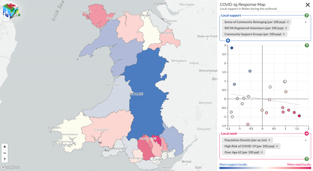
Screenshot from the https://covidresponsemap.wales/ site.

Ensuring support is available where needed 

Community support can offer a protective factor against adverse events. Some areas are more vulnerable than others, but knowing which areas are most likely to have a mismatch between support needed and support offered is difficult. To address this issue, a collaboration between the Public Health Wales Research & Evaluation Division and the Dynamic Genetics lab, part of the MRC Integrative Epidemiology Unit at the University of Bristol and supported by the Alan Turing Institute, has mapped these support offers and needs 

Using data from Wales Council for Voluntary Action, COVID-19 Mutual Aid, Welsh Government Statistics and Research, the Office for National Statistics, and social media the project team have created a live map that highlights the areas where further support for communities may be needed. It shows data on support factors, such as number of registered volunteers and population density, against risks, such as demographics, levels of deprivation, and internet access. It aims to inform the responses of national and local government, as well as support providers in Wales. 

The site also provides the links to local community groups identified helping to raise awareness of the support available locally. 

This map is part of an effort to better understand which communities have better community cohesion and organisation. We are keen to find out your views on how this can be more useful, or other community mobilisation data sources which could be included. Please contact Oliver or Nina with your comments: 

Dr Oliver Davis: oliver.davis@bristol.ac.uk  

Nina Di Cara nina.dicara@bristol.ac.uk 


Further information 


Are teachers at high risk of death from Covid19?

Sarah Lewis, George Davey Smith and Marcus Munafo

Follow Sarah, George and Marcus on Twitter

Due to the SARS-CoV-2 pandemic schools across the United Kingdom were closed to all but a small minority of pupils (children of keyworkers and vulnerable children) on the 20th March 2020, with some schools reporting as few as 5 pupils currently attending. The UK government have now issued guidance that primary schools in England should start to accept pupils back from the 1st June 2020 with a staggered return, starting with reception, year 1 and year 6.

Concern from teachers’ unions

This has prompted understandable concern from the  teachers’ unions, and on the 13th May, nine unions which represent teachers and education professionals signed a joint statement calling on the government to postpone reopening school on the 1st June, “We all want schools to re-open, but that should only happen when it is safe to do so. The government is showing a lack of understanding about the dangers of the spread of coronavirus within schools, and outwards from schools to parents, sibling and relatives, and to the wider community.” At the same time, others have suggested that the harms to many children due to neglect, abuse and missed educational opportunity arising from school closures outweigh the small increased risk to children, teachers and other adults of catching the virus.

What risk does Covid19 pose to children?

Weighing up the risks to children and teachers

So what do we know about the risk to children and to teachers? We know that children are about half as likely to catch the virus from an infected person as adults, and  if they do catch the virus they  are likely to have only mild symptoms.  The current evidence, although inconclusive, also suggests that they may be less likely to transmit the virus than adults.  However, teachers have rightly pointed out that there is a risk of transmission between the teachers themselves and between parents and teachers.

The first death from COVID-19 in England was recorded at the beginning of March 2020 and by the 8th May 2020 39,071 deaths involving COVID-19 had been reported in England and Wales. Just three of these deaths were among children aged under 15 years and  only a small proportion of the deaths (4416 individuals, 11.3%) were among working aged people.  Even among this age group risk is not uniform; it increases sharply with age from 2.6 in 100,000 for 25-44 years olds with a ten fold increase to 26 in  100,000 individuals for those aged 45-64.

Risks to teachers compared to other occupations

In addition, each underlying health condition increases the risk of dying from COVID-19, with those having at least 1 underlying health problem making up most cases.   The Office for National Statistics in the UK have published age standardised deaths by occupation for all deaths involving COVID-19 up to the 20th April 2020. Most of the people dying by this date would have been infected at the peak of the pandemic in the UK  prior to the lockdown period. They found that during this period there were 2494 deaths involving Covid-19 in the working age population. The mortality rate for Covid-19 during this period was 9.9 (95% confidence intervals 9.4-10.4) per 100,000 males and 5.2 (95%CI 4.9-5.6) per 100,000 females, with Covid-19 involved in around 1 in 4 and 1 in 5 of all deaths among males and females respectively.

Amongst teaching and education professionals (which includes school teachers, university lecturers and other education professionals) a total of 47 deaths (involving Covid-19) were recorded, equating to mortality rates of 6.7 (95%CI 4.1-10.3) per 100,000 among males and 3.3 (95%CI 2.0-4.9) per 100,000 among females, which was very similar to the rates of 5.6 (95%CI 4.6-6.6) per 100,000 among males and 4.2(95%CI 3.3-5.2) per 100,000 females for all professionals. The mortality figures for all education professionals includes 7 out of 437000 (or 1.6 per 100,000 teachers) primary and nursery school teachers and 17 out of 395000 (or 4.3 per 100,000 teachers) secondary school teachers.  A further 20 deaths occurred amongst childcare workers giving a mortality rate amongst this group of 3.4 (95%CI=2.0-5.5) per 100,000 females (males were highly underrepresented in this group), this is in contrast to rates of 6.5 (95%CI=4.9-9.1) for female sales assistants and 12.7(95%CI= 9.8-16.2) for female care home workers.

Covid-19 risk does not appear greater for teachers than other working age individuals

In summary, based on current evidence the risk to teachers and childcare workers within the UK from Covid-19 does not appear to be any greater than for any other group of working age individuals. However, perceptions of elevated risk may have occurred, prompting some to ask “Why are so many teachers dying?” due to the way this issue is portrayed in the media with headlines such as “Revealed: At least 26 teachers have died from Covid-19” currently on the https://www.tes.com website. This kind of reporting, along with the inability of the government to communicate the substantial differences in risk between different population groups – in particular according to age – has caused understandable anxiety among teachers. Whilst, some teachers may not be prepared to accept any level of risk of becoming infected with the virus whilst at work, others may be reassured that the risk to them is small, particularly given that we all accept some level of risk in our lives, a value that can never be zero.

Likely impact on transmission in the community is unclear

As the majority of parents or guardians of school aged children will be in the 25-45 age range, the risk to them  is also likely to be small. Questions remain however around the effect of school openings on transmission in the community and the associated risk. This will be affected by many factors including the existing infection levels in the community, the extent to which pupils, parents and teachers are mixing outside of school (and at the school gate) and mixing between individuals of different age groups. This is the primary consideration of the government Scientific Advisory Group for Emergencies (SAGE) who are using modelling based on a series of assumptions to determine the effect of school openings on R0.


Sarah Lewis is a Senior Lecturer in Genetic Epidemiology in the department of Population Health Sciences, and is an affiliated member of the MRC Integrative Epidemiology Unit (IEU), University of Bristol

George Davey Smith is a Professor of Clinical Epidemiology, and director of the MRC IEU, University of Bristol

Marcus Munafo is a Professor of Biological Psychology, in the School of Psychology Science and leads the Causes, Consequences and Modification of Health Behaviours programme of research in the IEU, University of Bristol.


Collider bias: why it’s difficult to find risk factors or effective medications for COVID-19 infection and severity

Dr Gemma Sharp and Dr Tim Morris

Follow Gemma and Tim on twitter


The COVID-19 pandemic is proving to be a period of great uncertainty. Will we get it? If we get it, will we show symptoms? Will we have to go to hospital? Will we be ok? Have we already had it?

These questions are difficult to answer because, currently, not much is known about who is more at risk of being infected by coronavirus, and who is more at risk of being seriously ill once infected.

Researchers, private companies and government health organisations are all generating data to help shed light on the factors linked to COVID-19 infection and severity. You might have seen or heard about some of these attempts, like the COVID-19 Symptom Tracker app developed by scientists at King’s College London, and the additional questions being sent to people participating in some of the UK’s biggest and most famous health studies, like UK Biobank and the Avon Longitudinal Study of Parents and Children (ALSPAC).

These valuable efforts to gather more data will be vital in providing scientific evidence to support new public health policies, including changes to the lockdown strategy. However, it’s important to realise that data gathered in this way is ‘observational’, meaning that study participants provide their data through medical records or questionnaires but no experiment (such as comparing different treatments) is performed on them. The huge potential impact of COVID-19 data collection efforts makes it even more important to be aware of the difficulties of using observational data.

Image by Engin Akyurt from Pixabay

Correlation does not equal causation (the reason observational epidemiology is hard)

These issues boil down to one main problem with observational data: that it is difficult to tease apart correlation from causation.

There are lots of factors that correlate but clearly do not actually have any causal effect on each other. Just because, on average, people who engage in a particular behaviour (like taking certain medications) might have a higher rate of infection or severe COVID-19 illness, it doesn’t necessarily mean that this behaviour causes the disease. If the link is not causal, then changing the behaviour (for example, changing medications) would not change a person’s risk of disease. This means that a change in behaviour would provide no benefit, and possibly even harm, to their health.

This illustrates why it’s so important to be sure that we’re drawing the right conclusions from observational data on COVID-19; because if we don’t, public health policy decisions made with the best intentions could negatively impact population health.

Why COVID-19 research participants are not like everyone else

One particular issue with most of the COVID-19 data collected so far is that the people who have contributed data are not a randomly drawn or representative sample of the broader general population.

Only a small percentage of the population are being tested for COVID-19, so if research aims to find factors associated with having a positive or negative test, the sample is very small and not likely to be representative of everyone else. In the UK, people getting the test are likely to be hospital patients who are showing severe symptoms, or healthcare or other key workers who are at high risk of infection and severe illness due to being exposed to large amounts of the virus. These groups will be heavily over-represented in COVID-19 research, and many infected people with no or mild symptoms (who aren’t being tested) will be missed.

Aside from using swab tests, researchers can also identify people who are very likely to have been infected by asking about classic symptoms like a persistent dry cough and a fever. However, we have to consider that people who take part in these sorts of studies are also not necessarily representative of everyone else. For example, they are well enough to fill in a symptom questionnaire. They also probably use social media, where they likely found out about the study. They almost certainly own a smartphone as they were able to download the COVID-19 Symptom Tracker app, and they are probably at least somewhat interested in their health and/or in scientific research.

Why should we care about representativeness?

The fact that people participating in COVID-19 research are not representative of the whole population leads to two problems, one well-known and one less well-known.

Firstly, as often acknowledged by researchers, research findings might not be generalisable to everyone in the population. Correlations or causal associations between COVID-19 and the characteristics or behaviours of research participants might not exist amongst the (many more) people who didn’t take part in the research, but only in the sub-group who participated. So the findings might not translate to the general population: telling everyone to switch up their medications to avoid infection may only work for some people who are like those studied.

But there is a second problem, called ‘collider bias’ (sometimes also referred to using other names such as selection bias or sampling bias), that is less well understood and more difficult to grasp. Collider bias can distort findings so that certain factors appear related even when there is no relationship in the wider population. In the case of COVID-19 research, relationships between risk factors and infection (or severity of infection) can appear related when no causal effect exists, even within the sample of research participants.

As an abstract example, consider a private school where pupils are admitted only if they have either a sports scholarship or an academic scholarship. If a pupil at this school is not good at sports, we can deduce that they must be good at academic work. This correlation between being poor at sports but being good academically doesn’t exist in the real world outside of this school, but in the sample of school pupils, it appears. And so, with COVID-19 research, in the sample of people included in a COVID-19 dataset (e.g. people who have had a COVID-19 test), two factors that influence inclusion (e.g. having COVID-19 symptoms that were severe enough to warrant hospitalisation, and taking medications for a health condition that puts you at high risk of dying from COVID-19) would appear to be associated, even when they are not. That is, to be in the COVID-19 dataset (to be tested), people are likely to have had either more severe symptoms or to be on medication. The erroneous conclusion would follow that changing one factor (e.g. changing or stopping medications) would affect the other (i.e. lower the severity of COVID-19). Because symptom severity is related to risk of death, stopping medication would appear to reduce the chance of death. As such, any resulting changes to clinical practice would be ineffective or even harmful.

Policymaking is a complex process at the best of times, involving balancing evidence from research, practice, and personal experience with other constraints and drivers, such as resource pressures, politics, and values. Add into that the challenge of making critical decisions with incomplete information under intense time pressure, and the need for good quality evidence becomes even more acute. The expertise of statisticians, who can double check analyses and ensure that conclusions are as robust as possible, should be a central part of the decision making process at this time – and especially to make sure that erroneous conclusions arrived at as a result of collider bias do not translate into harmful practice for people with COVID-19.


*****************************************************************************************************

The main aim of this blog post was to highlight the issue of collider bias, which is notoriously tricky to grasp. We hope we’ve done this but would be interested in your comments.

For those looking for more information, read on to discover some of the statistical methods that can be used to address collider bias….

Now we know collider bias is a problem: how do we fix it?

It is important to consider the intricacies of observational data and highlight the very real problems that can arise from opportunistically collected data.  However, this needs to be balanced against the fact that we are in the middle of a pandemic, that important decisions need to be made quickly, and this data is all we have to guide decisions. So what can we do?

There are a few strategies, developed by statisticians and other researchers in multiple fields, that should be considered when conducting COVID-19 research:

  •       Estimate the extent of the collider bias:

o  Think about the profile of people in COVID-19 samples – are they older/younger or more/less healthy than individuals in the general population?

o Are there any unexpected correlations in the sample that ring alarm bells?

  • Try to balance out the analysis by ‘weighting’ individuals, so that people from under-represented groups count more than people from over-represented groups.
  • Carry out additional analysis, known as ‘sensitivity analysis’, to assess the extent to which plausible patterns of sample selection could alter measured associations.

For those who would like to read even more, here’s a pre print on collider bias published by our team:

Gareth GriffithTim T MorrisMatt TudballAnnie HerbertGiulia MancanoLindsey PikeGemma C SharpTom M PalmerGeorge Davey SmithKate TillingLuisa ZuccoloNeil M DaviesGibran Hemani


New evidence on risks of low-level alcohol use in pregnancy

Dr Kayleigh Easey (@KayEasey), from the Bristol Medical School’s MRC Integrative Epidemiology Unit at the University of Bristol, takes a look at a recent research investigating effects of drinking in pregnancy and child mental health.

Whilst it’s generally known that heavy alcohol use during pregnancy can cause physical and cognitive impairments in offspring, there has been relatively limited evidence about the effects of low to moderate alcohol use. As such there have been conflicting conclusions about the potential harm of drinking in pregnancy, and debate around official guidance.

Alcohol use in pregnancy is still common with a recent meta-analysis showing over 40% of women within the UK to have drank some alcohol whilst pregnant. In 2016 the Department of Health updated their guidance advising abstinence from alcohol throughout pregnancy. This was in contrast to their previous advice of abstaining from alcohol in the first three months, but that 1-2 units of alcohol per week were not likely to cause harm. The updated guidance reflected a precautionary approach based on researcher’s advice of ‘absence of evidence not being evidence of absence’, due to the challenges faced in this area of study.

Certainly it has been challenging for researchers to determine any causal effect of alcohol use in pregnancy, particularly as the existing observational studies do not show evidence of causality. As such, caution over interpretation of results is needed given the sensitivity of alcohol as a risk factor and traditional attitudes towards low-level drinking.

Our new research sought to add to the limited body of evidence investigating causal effects, specifically on how low to moderate alcohol use could influence offspring mental health. We used data from a longitudinal birth cohort (the Avon Longitudinal Study of Parents and Children) which has followed pregnant mothers, their partners and their offspring since the 1990s, to investigate whether the frequency mothers and their partners drank alcohol during pregnancy was associated with offspring depression at age 18. We also included partner’s alcohol use in pregnancy (which is unlikely to have a direct biological effect on the developing fetus) and were able to examine if associations were likely to be causal, or due to shared confounding factors between parents such as socio-demographic factors.

We found that children whose mothers drank any alcohol at 18 weeks pregnancy may have up to a 17% higher risk of depression at age 18 compared to those mothers who did not drink alcohol. What was really interesting here is that we also investigated paternal alcohol use during pregnancy and did not find a similar association. This suggests that the associations seen with maternal drinking may be causal, rather than due to confounding by other factors (which might be expected to be similar between mothers and their partners). Many of the indirect factors that could explain the maternal effects are shared between mothers and partners (such as socio-demographic factors); despite this, we only found associations for mothers drinking.

These findings suggest evidence of a likely causal effect from alcohol consumption during pregnancy, and therefore evidence to support the updated government advice that the safest approach for alcohol use during pregnancy is for abstinence. This adds to other limited research on the effects of low level alcohol use in pregnancy. Whilst further research is needed, women can use this information to further inform their choices and help avoid risk from alcohol use both during pregnancy and as a precautionary measure when trying to conceive, as supported by the #Drymester campaign.

Our study highlights also the importance of including partner behaviours during pregnancy to aid in identifying causal relationships with offspring outcomes, and also because these may be important in their own right. I am currently working within the EPoCH project (Exploring Parental Influences on Childhood Health) which investigates whether and how both maternal and paternal behaviours might impact childhood health. In the meantime, it may be time for a further public health promotion highlighting that an alcohol-free pregnancy really is safer for children’s health.


This post was originally published on the Alcohol Policy blog.

What can genetics tell us about how sleep affects our health?

Deborah Lawlor, Professor of Epidemiology, Emma Anderson, MRC Research Fellow, Marcus Munafò, Professor of Experimental Psychology, Mark Gibson, PhD student, Rebecca Richmond, Vice Chancellor’s Research Fellow

Follow Deborah, Marcus, and Rebecca on Twitter

Association is not causation – are we fooled (confounded) when we see associations between sleep problems and disease?

Sleep is important for health. Observational studies show that people who report having sleep problems are more likely to be overweight, and have more health problems including heart disease, some cancers and mental health problems.

A major problem with conventional observational studies is that we cannot tell whether these associations are causal; does being overweight cause sleep problems, or do sleep problems cause people to become overweight? Alternatively, factors that influence how we sleep may also influence our health. For example, smoking might cause sleep problems as well as heart disease and so we are fooled (confounded) into thinking sleep problems cause heart disease when it is really all explained by smoking. In the green paper Advancing our Health: Prevention in the 2020s, the UK Government acknowledged that sleep has had little attention in policy, and that causality between sleep and health is likely to run in both directions.

But, how can we determine the direction of causality for sure? And, how do we make sure we are results are not confounded?

Randomly allocated genetic variation

Our genes are randomly allocated to us from our parents when we are conceived. They do not change across our lifespan, and cannot be changed by smoking, overweight or ill health.

Here at the MRC Integrative Epidemiology Unit we have developed a research method called Mendelian randomization, which uses this family-level random allocation of genes to explore causal effects. To find out more about Mendelian randomization take a look at this primer from the Director of the Unit (Prof George Davey Smith).

In the last two years, we and colleagues from the Universities of Manchester, Exeter and Harvard have identified large numbers of genetic variants that relate to different sleep characteristics. These include:

  • Insomnia symptoms
  • How long, on average, someone sleeps each night
  • Chronotype (whether someone is an ‘early bird’ or ‘lark’ and prefers mornings, or a ‘night owl’ and prefers evenings). Chronotype is thought to reflect variation in our body clock (known as circadian rhythms).

We can use these genetic variants in Mendelian randomization studies to get a better understanding of whether sleep characteristics affect health and disease.

What we did

In our initial studies we used Mendelian randomization to explore the effects of sleep duration, insomnia and chronotype on body mass index, coronary heart disease, mental health problems, Alzheimer’s disease, and breast cancer. We analysed whether the genetic traits that are related to sleep characteristics – rather than the sleep characteristics themselves – are associated with the health outcomes. We combined those results with the effect of the genetic variants on sleep traits which allows us to estimate a causal effect. Using genetic variants rather than participants’ reports of their sleep characteristics makes us much more certain that the effects we identify are not due to confounding or reverse causation.

Are you a night owl or a lark?

What we found

Our results show a mixed picture; different sleep characteristics have varying effects on a range of health outcomes.

What does this mean?

Having better research evidence about the effects of sleep traits on different health outcomes means that we can give better advice to people at risk of specific health problems. For example, developing effective programmes to alleviate insomnia may prevent coronary heart disease and depression in those at risk. It can also help reduce worry about sleep and health, by demonstrating that some associations that have been found in previous studies are not likely to reflect causality.

If you are worried about your own sleep, the NHS has some useful guidance and signposting to further support.

Want to find out more?

Contact the researchers

Deborah A Lawlor mailto:d.a.lawlor@bristol.ac.uk

Further reading

This research has been published in the following open access research papers:

Genome-wide association analyses of chronotype in 697,828 individuals provides insights into circadian rhythms. Nature Comms (2019) https://www.nature.com/articles/s41467-018-08259-7

Biological and clinical insights from genetics of insomnia symptoms.  Nature Gen. (2019) https://www.ncbi.nlm.nih.gov/pmc/articles/PMC6415688/

Genome-wide association study identifies genetic loci for self-reported habitual sleep duration supported by accelerometer-derived estimates. Nature Comms. (2019) https://www.nature.com/articles/s41467-019-08917-4

Investigating causal relations between sleep traits and risk of breast cancer in women: mendelian randomisation study. BMJ (2019) https://www.bmj.com/content/365/bmj.l2327

Is disrupted sleep a risk factor for Alzheimer’s disease? Evidence from a two-sample Mendelian randomization analysis. https://www.biorxiv.org/content/10.1101/609834v1 (open access pre-print)

Evidence for Genetic Correlations and Bidirectional, Causal Effects Between Smoking and Sleep Behaviors. Nicotine and Tobacco (2018) https://www.ncbi.nlm.nih.gov/pmc/articles/PMC6528151/

Do development indicators underlie global variation in the number of young people injecting drugs?

Dr Lindsey Hines, Sir Henry Wellcome Postdoctoral Fellow in The Centre for Academic Mental Health & the Integrative Epidemiology Unit, University of Bristol

Dr Adam Trickey, Senior Research Associate in Population Health Sciences, University of Bristol

Follow Lindsey on Twitter

Injecting drug use is a global issue: around the world an estimated 15.6 million people inject psychoactive drugs. People who inject drugs tend to begin doing so in adolescence, and countries that have larger numbers of adolescents who inject drugs may be at risk of emerging epidemics of blood borne viruses unless they take urgent action. We mapped the global differences in the proportion of adolescents who inject drugs, but found that we may be missing the vital data we need to protect the lives of vulnerable young people. If we want to prevent HIV, hepatitis C, and overdose from sweeping through a new generation of adolescents we urgently need many countries to scale up harm reduction interventions, and to collect accurate which can inform public health and policy.

People who inject drugs are engaging in a behaviour that can expose them to multiple health risks such as addiction, blood-borne viruses, and overdose, and are often stigmatised. New generations of young people are still starting to inject drugs, and young people who inject drugs are often part of other vulnerable groups.

Much of the research into the causes of injecting drug use focuses on individual factors, but we wanted to explore the effect of global development on youth injecting. A recent systematic review showed wide country-level variation in the number of young people who comprise the population of people who inject drugs. By considering variation in countries, we hoped to be able to inform prevention and intervention efforts.

It’s important to note that effective interventions can reduce the harms of injecting drug use. Harm reduction programmes provide clean needles and syringes to reduce transmission of blood borne viruses. Opiate substitution therapy seeks to tackle the physical dependence on opiates that maintains injecting behaviour and has been shown to improve health outcomes.

What we did

Through a global systematic review and meta-analysis we aimed to find data on injecting drug use in published studies, public health and policy documents from every country. We used these data to estimate the global percentage of people who inject drugs that are aged 15-25 years old, and also estimated this for each region and country. We wanted to understand what might underlie variation in the number of young people in populations of people who inject drugs, and so we used data from the World Bank to identify markers of a country’s wealth, equality, and development.

What we found

Our study estimated that, globally, around a quarter of people who inject drugs are adolescents and young adults. Applied to the global population, we can estimate approximately 3·9 million young people inject drugs. As a global average, people start injecting drugs at 23 years old.

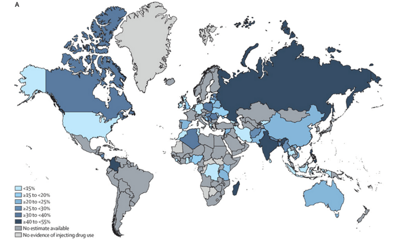
Estimated percentage of young people amongst those who inject drugs in each country

We found huge variation in the percentage of young people in each country’s population of people who inject drugs. Regionally, Eastern Europe had the highest proportion of young people amongst their populations who inject drugs, and the Middle Eastern and North African region had the lowest. In both Russia and the Philippines, over 50% of the people who inject drugs were aged 25 or under, and the average age of the populations of people who inject drugs was amongst the lowest observed.

Average age of the population of people who inject drugs in each country

In relation to global development indicators, people who inject drugs were younger in countries with lower wealth (indicated through Gross Domestic Product per capita) had been injecting drugs for a shorter time period. In rapidly urbanising countries (indicated through urbanisation growth rate) people were likely to start injecting drugs at later ages than people in countries with a slower current rate of urbanisation. We didn’t find any relationships between the age of people who inject drugs and a country’s youth unemployment, economic equality, or level provision of opiate substitution therapy.

However, many countries were missing data on injecting age and behaviours, or injecting drug use in general, which could affect these results.

What this means

1. The epidemic of injecting drug use is being maintained over time.

A large percentage of people who inject drugs are adolescents, meaning that a new generation are being exposed to the risks of injecting – and we found that this risk was especially high in less wealthy countries.

2. We need to scale up access to harm reduction interventions

There are highly punitive policies towards drug use in the countries with the largest numbers of young people in their populations of people who inject drugs. Since 2016, thousands of people who use drugs in the Philippines have died at the hands of the police. In contrast, Portugal has adopted a public health approach to drug use and addiction for decades, taking the radical step of taking people caught with drugs or personal use into addiction services rather than prisons. The rate of drug-related deaths and HIV infections in Portugal has since plummeted, as has the overall rate of drug use amongst young people: our data show that Portugal has a high average age for its population of people who inject drugs. If we do not want HIV, hepatitis C, and drug overdoses to sweep through a new generation of adolescents, we urgently need to see more countries adopting the approach pioneered by Portugal, and scaling up access to harm reduction interventions to the levels recommended by the WHO.

3. We need to think about population health, and especially mental health, alongside urban development.

Global development appears to be linked to injecting drug use, and the results suggest that countries with higher urbanisation growth are seeing new, older populations beginning to inject drugs. It may be that changes in environment are providing opportunities for injecting drug use that people hadn’t previously had. It’s estimated that almost 70% of the global population will live in urban areas by 2050, with most of this growth driven by low and middle-income countries.

4. We need to collect accurate data

Despite the health risks of injecting drug use, and the urgent need to reduce risks for new generations, our study has revealed a paucity of data monitoring this behaviour. Most concerning, we know the least about youth injecting drug use in low- and middle-income countries: areas likely to have the highest numbers of young people in their populations of people who inject drugs. Due to the stigma and the illicit nature of injecting drug use it is often under-studied, but by failing to collect accurate data to inform public health and policy we are risking the lives of vulnerable young people.

Contact the researchers

Lindsey.hines@bristol.ac.uk

Lindsey is funded by the Wellcome Trust.

Beyond question: a collaboration between EPoCH and artist Olga Trevisan

Back in May, IEU researcher Dr Gemma Sharp took part in Creative Reactions, an initiative that pairs scientists with artists to create artwork based on their academic research. With 50 artists and 50 scientists collaborating on works from sculptures and wood carvings to canvas, digital and performance art, the 2019 exhibition ran across two venues in Bristol.

Gemma was paired with Olga Trevisan, an artist based in Venice, Italy. They had conversations over Skype where they spoke about their work and formed some initial ideas about how they could combine their interests in a new way while remaining coherent to their own practices. Reflecting on the collaboration, Olga said, “I love how curious you can be of a subject you haven’t considered before. I believe collaboration helps to open your own mind.”

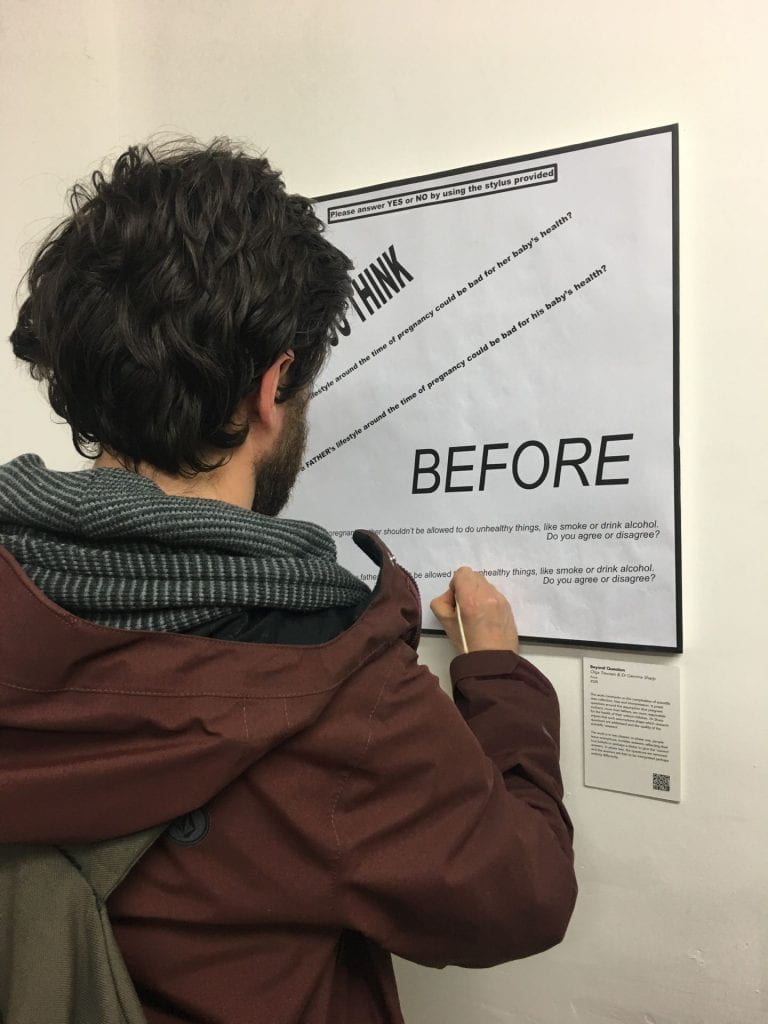
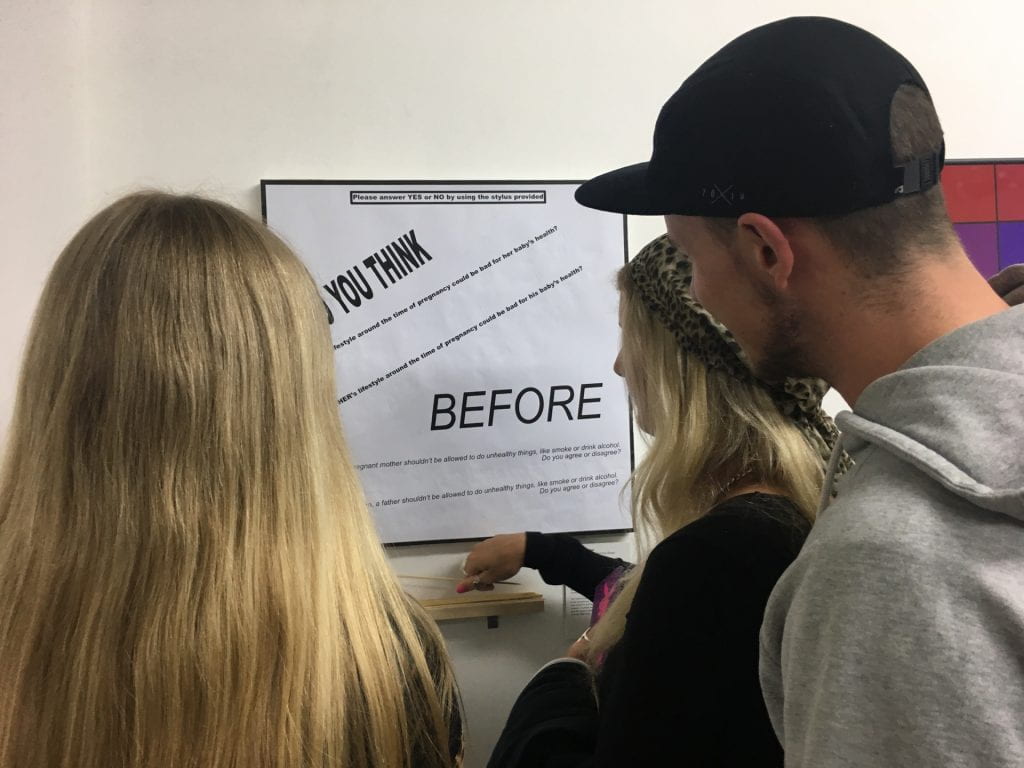
Based on some of the work around EPoCH, Olga created a piece called Beyond Question, which comments on the complexities of scientific data collection, bias and interpretation.

It poses questions around the pervasive assumption that pregnant women are more responsible for the (ill) health of their unborn children than their male partners are. Gemma and colleagues have argued that such assumptions drive the research agenda and the public perception of parental roles, by shaping which research questions get asked, which data are collected, and the quality of the scientific ‘answer’.

Photo credit: Olga Trevisan

Beyond Question was presented in two phases at two separate exhibitions: during the first phase, people were invited to answer questions with a simple Yes or No using a stylus; leaving no marks but only invisible, anonymous traces on the surface below. Answers will reflect the real assumptions, beliefs and attitudes of the respondent, but perhaps also, despite anonymity, their eagerness to ‘please’ the questioners, to give the ‘right’ answer, and to mask their true responses to paint themselves in the ‘best’ light.

In the second phase, the questions were removed and the answer traces were left alone to carry their own meaning; free to be combined with the attitudes, beliefs and assumptions of the viewer and to be interpreted and judged in perhaps an entirely different way.

Photo credit: Olga Trevisan

The questions posed were:

  • “Do you think a mother’s lifestyle around the time of pregnancy could be bad for her baby’s health?”
  • “Do you think a father’s lifestyle around the time of pregnancy could be bad for his baby’s health?”
  • “Before her baby is born, a pregnant mother shouldn’t be allowed to do unhealthy things, like smoke or drink alcohol. Do you agree or disagree?”
  • “Before his baby is born, a father shouldn’t be allowed to do unhealthy things, like smoke or drink alcohol. Do you agree or disagree?”

Find out more

Further info about Creative Reactions Bristol is available on their facebook page, or contact Matthew Lee on matthew.lee@bristol.ac.uk 

This blog post was originally posted on the EPOCH blog.

Using evidence to advise public health decision makers: an insider’s view

This blog post reviews a recent seminar hosted by the MRC IEU, PolicyBristol and the Bristol Population Health Science Institute.

Public health is one of the most contested policy areas. It brings together ethical and political issues and evidence on what works, and affects us all as citizens.

Researchers produce evidence and decision-makers receive advice – but how does evidence become advice and who are the players who take research findings and present advice to politicians and budget-holders?

We were pleased to welcome a diverse audience of around 75 multidisciplinary academics, policymakers and practitioners to hear our seminar speakers give a range of insider perspectives on linking academic research with national and local decisions on what to choose, fund and implement.

In this blog post we summarise the seminar, including links to the slides and event recording.

Seminar audience
Seminar attendees in the Coutts lecture theatre. Image credit: Julio Hermosilla Elgueta

Chair David Buck from The King’s Fund opened the event, highlighting the importance of conversations between different sectors of the evidence landscape, and of local decision-making in this context.

‘The art of giving advice’

The session was kicked off by Richard Gleave, Deputy Chief Executive, Public Health England, who is also undertaking a PhD on how evidence is used in public health policy decision making.

His presentation ‘Crossing boundaries – undertaking knowledge informed public health’ set the context, observing that most academic teams – from microbiology labs to mental health researchers – aim to improve policy and practice; but ‘the art of giving advice is as important and challenging as the skill required to review the evidence’.

Richard then introduced a range of provocations and stereotypes about how the policy decision making process can be framed.

Citing Dr Kathryn Oliver, he encouraged attendees to challenge the idea that there’s an ‘evidence gap’ to be crossed, and instead focus on doing good working together to improve the public’s health.

Giving an example of the Institute for Government’s analysis of how the smoking ban was enacted, he noted the role of a small number of influential groups and individuals in securing a total ban in 2007. He encouraged actively crossing the boundaries between academia, policy and practice, and working with boundary organisations and influencers as part of this process.

‘Partnerships between science and society’

Professor Isabel Oliver gave a second national perspective.

Speaking as a research-active Director of Research, Translation and Innovation and Deputy Director of the National Infection Service, she suggested that ‘Partnerships between Science and Society’ are the key to evidence based public health.

She questioned why is it when we have such an abundance of research, we still don’t have the evidence we need? And why does it take so long to implement research findings? She argued that a key issue here is relevance; how relevant is the research being produced, especially to current policy priorities?

Isabel outlined challenges including:

  • Needing evidence quickly in response to public health emergencies, and not being able to access it, for example how to bottle-feed babies during flooding crises, or whether to close schools during flu pandemics
  • Mismatched policy and research priorities; e.g. policy needing evidence on the impact of advertising on childhood obesity, but research focusing on the genetics of obesity
  • The (unhelpful) prevalence of ‘more research needed’ as a conclusion, and knowing when the evidence is sufficient to make a decision
  • A need to develop trust between stakeholders, made more challenging by the frequency of policy colleagues moving roles.

She also questioned whether the paradigm of evidence-based medicine works for complex issues such as public health or environmental policy.

Isabel concluded with some observations; that broader and more collaborative research questions that address the real issues are needed; and collaborating with a broad range of stakeholders, including industry and finance, should not be discounted.

She finished by reiterating a call for public health advice that is relevant, and responds to a policy ‘window’ being open.

Seminar speakers L-R: Dr Olivia Maynard, Richard Gleave, Professor Isabel Oliver and Christina Gray. Image credit: Julio Hermosilla Elgueta

‘Local perspective’

Christina Gray, Director of Public Health at Bristol City Council gave the local view, providing a helpful explanation of her role and the process of decision making within a local authority.

She outlined three key principles:

  • The democratic principle; elected members are ‘the council’; officers (including her role) provide advice. Local authorities are close to their people and are publicly accountable. Their decisions are formally scrutinised and need to be justified, and resource allocation is a key – and stark – challenge, especially in the context of austerity.
  • The narrative principle: how the society that the authority represents holds multiple legitimate (and competing or conflicting) perspectives and realities, which all need to be considered.
  • The (social) scientific principle; the development of human knowledge in a systematic way – which is then shared into the democratic process, as one of a range of narratives.

Christina outlined a case study example of an initiative on period dignity which Bristol City Council is leading as part of Bristol’s One City Plan, and how the evidence base for the programme was located and used. She posed the question of what evidence matters locally, and suggested that evidence of impact, economic evidence, and retrospective evidence that demonstrates whether what has been done works, in order to build on it, are the most helpful. To close, Christina highlighted the importance of being ‘paradigm literate’ in order to navigate the complexity of public health decision making.

Academic perspective

Our final speaker, Dr Olivia Maynard, gave an academic perspective on how to advise decision makers.

Focusing on practical tips, she outlined her own work on tobacco, smoking, e-cigarettes, alcohol and other drugs and how she has engaged with various opportunities to work with policymakers.

Starting with a clear case for doing the work (it’s important, it’s interesting, to create impact), she went on to outline methods of engagement:

  • Proactively presenting your work; introduce yourself to policymakers interested in your area such as MPs, Peers, APPGs, subject specialists in parliamentary research services, advocacy groups, and PolicyBristol; review Hansard and Early Day Motions; get involved in parliamentary events
  • Respond to calls for evidence (University of Bristol researchers can find curated opportunities via the PolicyBristol PolicyScan)
  • Work directly with policymakers, for example via Policy Fellowships (for example with POST)

Olivia outlined some reflections around the differences between academia and policymaking.

Timelines for action is one, but she also used the changes towards plain packaging as an example to note that the policymaking process can span numerous years, presenting many opportunities for intervention.

She referred back to Christina’s point about ‘multiple competing realities’ to highlight that evidence is one of many factors to consider in policymaking.

She also encouraged academics to challenge ‘imposter syndrome’, by emphasising ‘you are more of an expert than you think you are’, and needing to make yourself known to be offered opportunities.

Where next?

Chair David Buck highlighted a number of themes running throughout the presentations including recognising the paradigms used by different stakeholders; questioning what counts as evidence, and being able to provide advice from an uncertain evidence base; and what these themes mean for all of us (and how willing are we to act on these reflections?)

The seminar concluded with a facilitated Q&A session spanning topics such as:

  • Should all research which influences policy be coproduced with user groups and policymakers?
  • What kind of ‘payback’ do stakeholder organisations need for their involvement in research projects?
  • How should researchers develop the skills needed to cross boundaries?
  • What funding is available for policy relevant research?
  • How can we make our evidence ‘stand out’?
  • Should academics have a responsibility to critique policy?

The seminar started numerous conversations which we hope to continue.

Chair David Buck facilitates our Q&A. Image credit: Julio Hermosilla Elgueta

Access the slides:

1. Richard Gleave Crossing boundaries – undertaking knowledge informed public health

2. Isabel Oliver Partnerships between science and society

3. Christina Gray Evidence into practice

4. Olivia Maynard An academic’s perspective

View a recording of the event on the IEU’s YouTube channel: https://www.youtube.com/watch?v=-ew-RvzV-D0 

Contact lindsey.pike@bristol.ac.uk if you’d like to hear about future events.


stopWatch – a smartwatch system that could help people quit smoking

Dr Andy Skinner and Chris Stone

Follow Andy and Chris on twitter


October sees the return of Stoptober, a Public Health England initiative to encourage smokers to quit. Campaigns like this and many others have been effective in reducing smoking in the UK over a number of decades. However, on average, about 15% of the UK’s population still smoke, and this costs the NHS more than £2.5bn each year.

To help address this, the NHS Long Term Plan has identified a range of measures to encourage healthier behaviours, including the need to speed up the introduction of innovative new health interventions based on digital technologies.

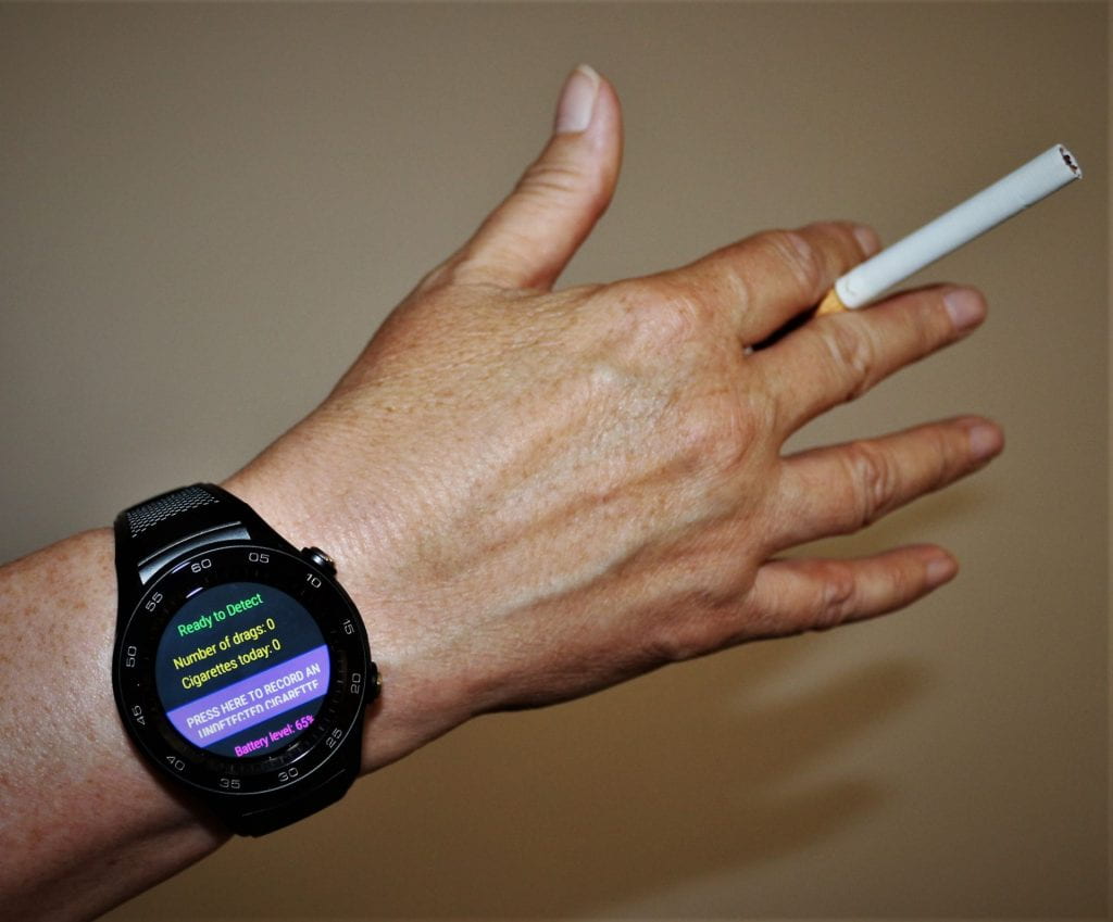
Here in the MRC IEU we’ve been working on a new wearable system that could help people stop smoking; stopWatch is a smartwatch-based system that automatically detects cigarette smoking. Because the system can detect when someone is smoking a cigarette, it can trigger the delivery of interventions to help that person quit smoking at precisely the time the interventions will be most effective.

Hand and wrist wearing stopWatch and holding a cigarette
The stopWatch could help people to stop smoking

What is stopWatch, and how does it work?

stopWatch is an application that runs on a commercially available Android smartwatch. Smartwatches now come equipped with motion sensors, just like the ones in smartphones that measure step counts and activity levels. As smartwatches are attached to the wrist, the motion sensors in a smartwatch can tell us how a person’s hand is moving. stopWatch takes data from the smartwatch’s motion sensors and applies machine learning methods to look for the particular pattern of hand movements that are unique to smoking a cigarette.

How can we use stopWatch to help people quit smoking?

It’s estimated about a third of UK smokers try to stop each year, but only a fifth of those that try manage to succeed. For most smokers an attempt to stop smoking ends with a lapse (having just one cigarette), that can quickly lead to a full relapse to smoking. As stopWatch can detect the exact moment a smoker lapses and has a cigarette, it can trigger the precise delivery of an intervention aimed specifically at helping prevent the lapse turning into a full relapse back to smoking.

Will the intervention work?

A recent article highlighted the potential for using mobile and wearable technologies, like stopWatch, to deliver these kinds of ‘just-in-time’ interventions for smoking. To develop our smoking relapse intervention we will be using the person-based approach, which has an excellent track record of delivering effective health behaviour change interventions. We will also be engaging the highly interdisciplinary cohort of PhD students in the new EPSRC Center for Doctoral Training in Digital Health and care, which brings together students with backgrounds in health, computer science, design and engineering.

However, that same article also pointed out that these types of intervention are still new, and that there has been little formal evaluation of them so far. So we don’t yet know how effective these will be, and it’s important interventions of this kind are subject to a thorough evaluation.

We will be working closely with colleagues in NIHR’s Applied Research Collaboration (ARC) West and Bristol Biomedical Research Centre who have expertise in developing, and importantly, evaluating interventions. We will also be working with the CRUK-funded Integrative Cancer Epidemiology Unit at the University of Bristol, collaborating with researchers who have detailed knowledge of developing interventions for specific patient groups.

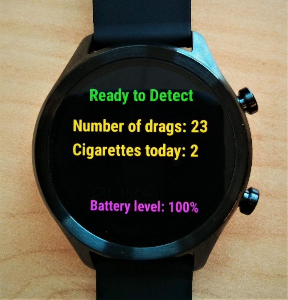
The StopWatch display
On average, stopWatch detected 71% of cigarettes smoked and of the events stopWatch thought were cigarette smoking, 86% were actually cigarette smoking.

How good is stopWatch at detecting cigarette smoking?

In any system designed to recognise behaviours there is a trade-off between performance and cost/complexity. Other systems that use wearables to detect smoking are available, but these require the wearable be paired with a smartphone and need a data connection to a cloud-based platform in order to work properly. stopWatch is different in that it runs entirely on a smartwatch. It doesn’t need to be paired with a smartphone, and doesn’t need a data connection. This makes it cheaper and simpler than the other systems, but this also means its performance isn’t quite as good.

We recently validated the performance of stopWatch by asking thirteen participants to use stopWatch for a day as they went about their normal lives. On average, stopWatch detected 71% of cigarettes smoked (the system’s sensitivity), and of the events stopWatch thought were cigarette smoking, 86% were actually cigarette smoking (its specificity). This compares with a sensitivity of 82% and specificity of 97% for the systems that require smartphones and data networks.

When will stopWatch and the smoking relapse intervention be available and what will they cost?

The stopWatch system itself is available for research purposes to academic partners now, free of charge. We’re open to discussions with potential commercial partners – please get in touch if you’d like to discuss this (contact details below).

We aim to begin work on the smoking relapse intervention based on stopWatch next year, and we expect development and evaluation to take between 18 and 24 months. The cost of the intervention has yet to be determined. That will depend on many factors, including the partnerships we form to take the intervention forward.

What’s next?

We’re currently putting stopWatch through its paces in some tough testing in occupational settings. This will stress the system so that we can identify any weaknesses, find out to how to improve the system, and develop recommendations for optimising the use of stopWatch in future studies and interventions.

We’re also developing a new smartwatch-based system for the low burden collection of self-report data called ‘dataWatch’. This is currently undergoing feasibility testing in the Children of the 90s study.

Contact the researchers

Dr Andy Skinner Andy.Skinner@bristol.ac.uk 

Social media in peer review: the case of CCR5

Last week IEU colleague Dr Sean Harrison was featured on BBC’s Inside Science, discussing his role in the CCR5-mortality story. Here’s the BBC’s synopsis:

‘In November 2018 news broke via YouTube that He Jiankui, then a professor at Southern University of Science and Technology in Shenzhen, China had created the world’s first gene-edited babies from two embryos. The edited gene was CCR5 delta 32 – a gene that conferred protection against HIV. Alongside the public, most of the scientific community were horrified. There was a spate of correspondence, not just on the ethics, but also on the science. One prominent paper was by Rasmus Nielsen and Xinzhu Wei’s of the University of California, Berkeley. They published a study in June 2019 in Nature Medicine that found an increased mortality rate in people with an HIV-preventing gene variant. It was another stick used to beat Jiankiu – had he put a gene in these babies that was not just not helpful, but actually harmful? However it now turns out that the study by Nielsen and Wei has a major flaw. In a series of tweets, Nielsen was notified of an error in the UK Biobank data and his analysis. Sean Harrison at the University of Bristol tried and failed to replicate the result using the UK Biobank data. He posted his findings on Twitter and communicated with Nielsen and Wei who have now requested a retraction. UCL’s Helen O’Neill is intimately acquainted with the story and she chats to Adam Rutherford about the role of social media in the scientific process of this saga.’

Below, we re-post Sean’s blog which outlines how the story unfolded, and the analysis that he ran.

Follow Sean on Twitter

Listen to Sean on Inside Science

*****************************************************************************************************************************************

“CCR5-∆32 is deleterious in the homozygous state in humans” – is it?

I debated for quite a long time on whether to write this post. I had said pretty much everything I’d wanted to say on Twitter, but I’ve done some more analysis and writing a post might be clearer than another Twitter thread.

To recap, a couple of weeks ago a paper by Xinzhu (April) Wei & Rasmus Nielsen of the University of California was published, claiming that a deletion in the CCR5 gene increased mortality (in white people of British ancestry in UK Biobank). I had some issues with the paper, which I posted here. My tweets got more attention than anything I’d posted before. I’m pretty sure they got more attention than my published papers and conference presentations combined. ¯\_(ツ)_/¯

The CCR5 gene is topical because, as the paper states in the introduction:

In late 2018, a scientist from the Southern University of Science and Technology in Shenzhen, Jiankui He, announced the birth of two babies whose genomes were edited using CRISPR

To be clear, gene-editing human babies is awful. Selecting zygotes that don’t have a known, life-limiting genetic abnormality may be reasonable in some cases, but directly manipulating the genetic code is something else entirely. My arguments against the paper did not stem from any desire to protect the actions of Jiankui He, but to a) highlight a peer review process that was actually pretty awful, b) encourage better use of UK Biobank genetic data, and c) refute an analysis that seemed likely biased.

This paper has received an incredible amount of attention. If it is flawed, then poor science is being heavily promoted. Apart from the obvious problems with promoting something that is potentially biased, others may try to do their own studies using this as a guideline, which I think would be a mistake.
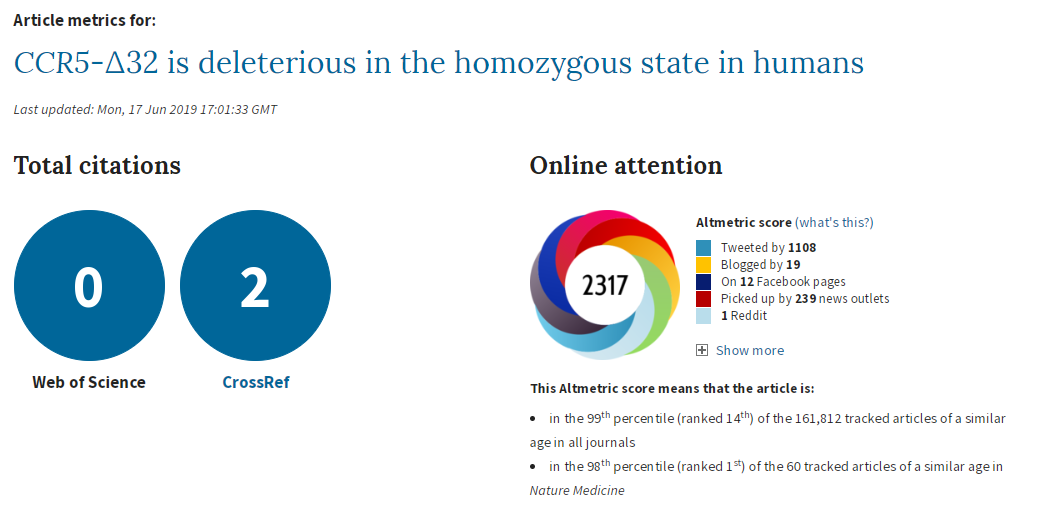
1

I’ll quickly recap the initial problems I had with the paper (excluding the things that were easily solved by reading the online supplement), then go into what I did to try to replicate the paper’s results. I ran some additional analyses that I didn’t post on Twitter, so I’ll include those results too.

Full disclosure: in addition to tweeting to me, Rasmus and I exchanged several emails, and they ran some additional analyses. I’ll try not to talk about any of these analyses as it wasn’t my work, but, if necessary, I may mention pertinent bits of information.

I should also mention that I’m not a geneticist. I’m an epidemiologist/statistician/evidence synthesis researcher who for the past year has been working with UK Biobank genetic data in a unit that is very, very keen on genetic epidemiology. So while I’m confident I can critique the methods for the main analyses with some level of expertise, and have spent an inordinate amount of time looking at this paper in particular, there are some things where I’ll say I just don’t know what the answer is.

I don’t think I’ll write a formal response to the authors in a journal – if anyone is going to, I’ll happily share whatever information you want from my analyses, but it’s not something I’m keen to do myself.

All my code for this is here.

The Issues

Not accounting for relatedness

Not accounting for relatedness (i.e. related people in a sample) is a problem. It can bias genetic analyses through population stratification or familial structure, and can be easily dealt with by removing related individuals in a sample (or fancy analysis techniques, e.g. Bolt-LMM). The paper ignored this and used everyone.

Quality control

Quality control (QC) is also an issue. When the IEU at the University of Bristol was QCing the UK Biobank genetic data, they looked for sex mismatches, sex chromosome aneuploidy (having sex chromosomes different to XX or XY), and participants with outliers in heterozygosity and missing rates (yeah, ok, I don’t have a good grasp on what this means, but I see it as poor data quality for particular individuals). The paper ignored these too.

Ancestry definition

The paper states it looks at people of “British ancestry”. Judging by the number in participants in the paper and the reference they used, the authors meant “white British ancestry”. I feel this should have been picked up on in peer review, since the terms are different. The Bycroft article referenced uses “white British ancestry”, so it would have certainly been clearer sticking to that.

Covariable choice

The main analysis should have also been adjusted for all principal components (PCs) and centre (where participants went to register with UK Biobank). This helps to control for population stratification, and we know that UK Biobank has problems with population stratification. I thought choosing variables to include as covariables based on statistical significance was discouraged, but apparently I was wrong. Still, I see no plausible reason to do so in this case – principal components represent population stratification, population stratification is a confounder of the association between SNPs and any outcome, so adjust for them. There are enough people in this analysis to take the hit.

The analysis
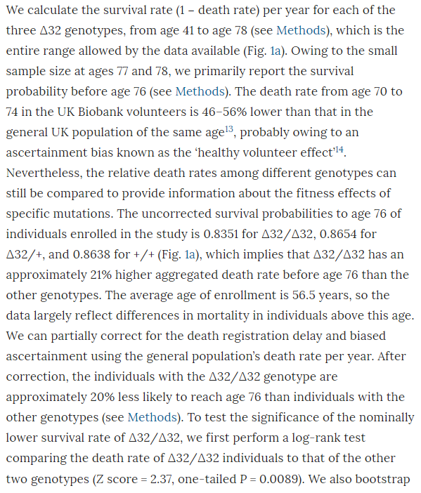
10

I don’t know why the main analysis was a ratio of the crude mortality rates at 76 years of age (rather than a Cox regression), and I don’t know why there are no confidence intervals (CIs) on the estimate. The CI exists, it’s in the online supplement. Peer review should have had problems with this. It is unconscionable that any journal, let alone a top-tier journal, would publish a paper when the main result doesn’t have any measure of the variability of the estimate. A P value isn’t good enough when it’s a non-symmetrical error term, since you can’t estimate the standard error.

So why is the CI buried in an additional file when it would have been so easy to put it into the main text? The CI is from bootstrapping, whereas the P value is from a log-rank test, and the CI of the main result crosses the null. The main result is non-significant and significant at the same time. This could be a reason why the CI wasn’t in the main text.

It’s also noteworthy that although the deletion appears strongly to be recessive (only has an effect is both chromosomes have the deletion), the main analysis reports delta-32/delta-32 against +/+, which surely has less power than delta-32/delta-32 against +/+ or delta-32/+. The CI might have been significant otherwise.
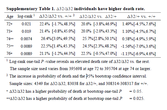
2

I think it’s wrong to present one-sided P values (in general, but definitely here). The hypothesis should not have been that the CCR5 deletion would increase mortality; it should have been ambivalent, like almost all hypotheses in this field. The whole point of the CRISPR was that the babies would be more protected from HIV, so unless the authors had an unimaginably strong prior that CCR5 was deleterious, why would they use one-sided P values? Cynically, but without a strong reason to think otherwise, I can only imagine because one-sided P values are half as large as two-sided P values.

The best analysis, I think, would have been a Cox regression. Happily, the authors did this after the main analysis. But the full analysis that included all PCs (but not centre) was relegated to the supplement, for reasons that are baffling since it gives the same result as using just 5 PCs.

Also, the survival curve should have CIs. We know nothing about whether those curves are separate without CIs. I reproduced survival curves with a different SNP (see below) – the CIs are large.
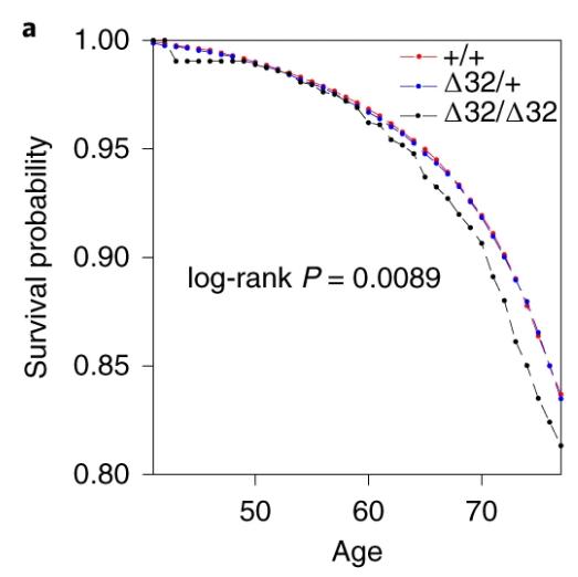
3

I’m not going to talk about the Hardy-Weinburg Equilibrium (HWE, inbreeding) analysis– it’s still not an area I’m familiar with, and I don’t really think it adds much to the analysis. There are loads of reasons why a SNP might be out of HWE – dying early is certainly one of them, but it feels like this would just be a confirmation of something you’d know from a Cox regression.

Replication Analyses

I have access to UK Biobank data for my own work, so I didn’t think it would be too complex to replicate the analyses to see if I came up with the same answer. I don’t have access to rs62625034, the SNP the paper says is a great proxy of the delta-32 deletion, for reasons that I’ll go into later. However, I did have access to rs113010081, which the paper said gave the same results. I also used rs113341849, which is another SNP in the same region that has extremely high correlation with the deletion (both SNPs have R2 values above 0.93 with rs333, which is the rs ID for the delta-32 deletion). Ideally, all three SNPs would give the same answer.

First, I created the analysis dataset:

  1. Grabbed age, sex, centre, principal components, date of registration and date of death from the UK Biobank phenotypic data
  2. Grabbed the genetic dosages of rs113010081 and rs113341849 from the UK Biobank genetic data
  3. Grabbed the list of related participants in UK Biobank, and our usual list of exclusions (including withdrawals)
  4. Merged everything together, estimating the follow-up time for everyone, and creating a dummy variable of death (1 for those that died, 0 for everyone else) and another one for relateds (0 for completely related people, 1 for those I would typically remove because of relatedness)
  5. Dropped the standard exclusions, because there aren’t many and they really shouldn’t be here
  6. I created dummy variables for the SNPs, with 1 for participants with two effect alleles (corresponding to a proxy for having two copies of the delta-32 deletion), and 0 for everyone else
  7. I also looked at what happened if I left the dosage as 0, 1 or 2, but since there was no evidence that 1 was any different from 0 in terms of mortality, I only reported the 2 versus 0/1 results

I conducted 12 analyses in total (6 for each SNP), but they were all pretty similar:

  1. Original analysis: time = study time (so x-axis went from 0 to 10 years, survival from baseline to end of follow-up), with related people included, and using age, sex, principal components and centre as covariables
  2. Original analysis, without relateds: as above, but excluding related people
  3. Analysis 2: time = age of participant (so x-axis went from 40 to 80 years, survival up to each year of life, which matches the paper), with related people included, and using sex, principal components and centre as covariables
  4. Analysis 2, without relateds: as above, but excluding related people
  5. Analysis 3: as analysis 2, but without covariables
  6. Analysis 3, without relateds: as above, but excluding related people

With this suite of analyses, I was hoping to find out whether:

  • either SNP was associated with mortality
  • including covariables changed the results
  • the time variable changed the results, and d) whether including relateds changed the results

Results

4

I found… Nothing. There was very little evidence the SNPs were associated with mortality (the hazard ratios, HRs, were barely different from 1, and the confidence intervals were very wide). There was little evidence including relateds or more covariables, or changing the time variable, changed the results.

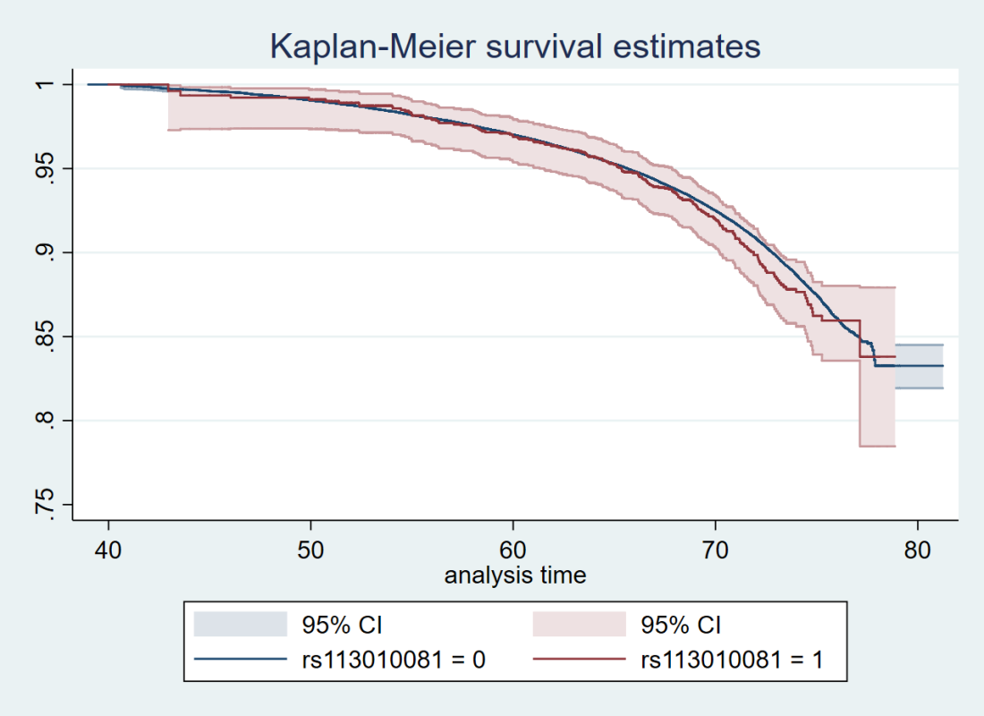
Here’s just one example of the many survival curves I made, looking at delta-32/delta-32 (1) versus both other genotypes in unrelated people only (not adjusted, as Stata doesn’t want to give me a survival curve with CIs that is also adjusted) – this corresponds to the analysis in row 6.
5

You’ll notice that the CIs overlap. A lot. You can also see that both events and participants are rare in the late 70s (the long horizontal and vertical stretches) – I think that’s because there are relatively few people who were that old at the end of their follow-up. Average follow-up time was 7 years, so to estimate mortality up to 76 years, I imagine you’d want quite a few people to be 69 years or older, so they’d be 76 at the end of follow-up (if they didn’t die). Only 3.8% of UK Biobank participants were 69 years or older.

In my original tweet thread, I only did the analysis in row 2, but I think all the results are fairly conclusive for not showing much.

In a reply to me, Rasmus stated:

6

This is the claim that turned out to be incorrect:

11

Never trust data that isn’t shown – apart from anything else, when repeating analyses and changing things each time, it’s easy to forget to redo an extra analysis if the manuscript doesn’t contain the results anywhere.

This also means I couldn’t directly replicate the paper’s analysis, as I don’t have access to rs62625034. Why not? I’m not sure, but the likely explanation is that it didn’t pass the quality control process (either ours or UK Biobank’s, I’m not sure).

SNPs

I’ve concluded that the only possible reason for a difference between my analysis and the paper’s analysis is that the SNPs are different. Much more different than would be expected, given the high amount of correlation between my two SNPs and the deletion, which the paper claims rs62625034 is measuring directly.

One possible reason for this is the imputation of SNP data. As far as I can tell, neither of my SNPs were measured directly, they were imputed. This isn’t uncommon for any particular SNP, as imputation of SNP data is generally very good. As I understand it, genetic code is transmitted in blocks, and the blocks are fairly steady between people of the same population, so if you measure one or two SNPs in a block, you can deduce the remaining SNPs in the same block.

In any case there is a lot of genetic data to start with – each genotyping chip measures hundred of thousands of SNPs. Also, we can measure the likely success rate of the imputation, and SNPs that are poorly imputed (for a given value of “poorly”) are removed before anyone sees them.

The two SNPs I used had good “info scores” (around 0.95 I think – for reference, we dropped all SNPs with an info score of less than 0.3 for SNPs with minor allele frequencies similar), so we can be pretty confident in their imputation. On the other hand, rs62625034 was not imputed in the paper, it was measured directly. That doesn’t mean everyone had a measurement – I understand the missing rate of the SNP was around 3.4% in UK Biobank (this is from direct communication with the authors, not from the paper).

But. And this is a weird but that I don’t have the expertise to explain, the imputation of the SNPs I used looks… well… weird. When you impute SNP data, you impute values between 0 and 2. They don’t have to be integer values, so dosages of 0.07 or 1.5 are valid. Ideally, the imputation would only give integer values, so you’d be confident this person had 2 mutant alleles, and this person 1, and that person none. In many cases, that’s mostly what happens.

Non-integer dosages don’t seem like a big problem to me. If I’m using polygenic risk scores, I don’t even bother making them integers, I just leave them as decimals. Across a population, it shouldn’t matter, the variance of my final estimate will just be a bit smaller than it should be. But for this work, I had to make the non-integer dosages integers, so anything less than 0.5 I made 0, anything 0.5 to 1.5 was 1, and anything above 1.5 was 2. I’m pretty sure this is fine.

Unless there’s more non-integer doses in one allele than the other.

rs113010081 has non-integer dosages for almost 14% of white British participants in UK Biobank (excluding relateds). But the non-integer dosages are not distributed evenly across dosages. No. The twos has way more non-integer dosages than the ones, which had way more non-integer dosages than the zeros.

In the below tables, the non-integers are represented by being missing (a full stop) in the rs113010081_x_tri variable, whereas the rs113010081_tri variable is the one I used in the analysis. You can see that of the 4,736 participants I thought had twos, 3,490 (73.69%) of those actually had non-integer dosages somewhere between 1.5 and 2.

7

What does this mean?

I’ve no idea.

I think it might mean the imputation for this region of the genome might be a bit weird. rs113341849 has the same pattern, so it isn’t just this one SNP.

But I don’t know why it’s happened, or even whether it’s particularly relevant. I admit ignorance – this is something I’ve never looked for, let alone seen, and I don’t know enough to say what’s typical.

I looked at a few hundred other SNPs to see if this is just a function of the minor allele frequency, and so the imputation was naturally just less certain because there was less information. But while there is an association between the minor allele frequency and non-integer dosages across dosages, it doesn’t explain all the variance in the estimate. There were very few SNPs with patterns as pronounced as in rs113010081 and rs113341849, even for SNPs with far smaller minor allele frequencies.

Does this undermine my analysis, and make the paper’s more believable?

I don’t know.

I tried to look at this with a couple more analyses. In the “x” analyses, I only included participants with integer values of dose, and in the “y” analyses, I only included participants with dosages < 0.05 from an integer. You can see in the results table that only using integers removed any effect of either SNP. This could be evidence that the imputation having an effect, or it could be chance. Who knows.

4

rs62625034

rs62625034 was directly measured, but not imputed, in the paper. Why?

It’s possibly because the SNP isn’t measuring what the probe meant to measure. It clearly has a very different minor allele frequency in UK Biobank (0.1159) than in the GO-ESP population (~0.03). The paper states this means it’s likely measuring the delta-32 deletion, since the frequencies are similar and rs62625034 sits in the deletion region. This mismatch may have made it fail quality control.

But this raises a couple of issues. First is whether the missingness in rs62625034 is a problem – is the data missing completely at random or not missing at random. If the former, great. If the latter, not great.

The second issue is that rs62625034 should be measuring a SNP, not a deletion. In people without the deletion, the probe could well be picking up people with the SNP. The rs62625034 measurement in UK Biobank should be a mixture between the deletion and a SNP. The R2 between rs62625034 and the deletion is not 1 (although it is higher than for my SNPs – again, this was mentioned in an email to me from the authors, not in the paper), which could happen if the SNP is picking up more than the deletion.

The third issue, one I’ve realised only just now, is that previous research has shown that rs62625034 is not associated with lifespan in UK Biobank (and other datasets). This means that maybe it doesn’t matter that rs62625034 is likely picking up more than just the deletion.

Peter Joshi, author of the article, helpfully posted these tweets:

89

If I read this right, Peter used UK Biobank (and other data) to produce the above plot showing lots of SNPs and their association with mortality (the higher the SNP, the more it affects mortality).

Not only does rs62625034 not show any association with mortality, but how did Peter find a minor allele frequency of 0.035 for rs62625034 and the paper find 0.1159? This is crazy. A minor allele frequency of 0.035 is about the same as the GO-ESP population, so it seems perfectly fine, whereas 0.1159 does not.

I didn’t clock this when I first saw it (sorry Peter), but using the same datasets and getting different minor allele frequencies is weird. Properly weird. Like counting the number of men and women in a dataset and getting wildly different answers. Maybe I’m misunderstanding, it wouldn’t be the first time – maybe the minor allele frequencies are different because of something else. But they both used UK Biobank, so I have no idea how.

I have no answer for this. I also feel like I’ve buried the lead in this post now. But let’s pretend it was all building up to this.

Conclusion

This paper has been enormously successful, at least in terms of publicity. I also like to think that my “post-publication peer review” and Rasmus’s reply represents a nice collaborative exchange that wouldn’t have been possible without Twitter. I suppose I could have sent an email, but that doesn’t feel as useful somehow.

However, there are many flaws with the paper that should have been addressed in peer review. I’d love to ask the reviewers why they didn’t insist on the following:

  • The sample should be well defined, i.e. “white British ancestry” not “British ancestry”
  • Standard exclusions should be made for sex mismatches, sex chromosome aneuploidy, participants with outliers in heterozygosity and missing rates, and withdrawals from the study (this is important to mention in all papers, right?)
  • Relatedness should either be accounted for in the analysis (e.g. Bolt-LMM) or related participants should be removed
  • Population stratification should be both addressed in the analysis (maximum principal components and centre) and the limitations
  • All effect estimates should have confidence intervals (I mean, come on)
  • All survival curves should have confidence intervals (ditto)
  • If it’s a survival analysis, surely Cox regression is better than ratios of survival rates? Also, somewhere it would be useful to note how many people died, and separately for each dosage
  • One-tailed P values need a huge prior belief to be used in preference to two-tailed P values
  • Over-reliance on P values in interpretation of results is also to be avoided
  • Choice of SNP, if you’re only using one SNP, is super important. If your SNP has a very different minor allele frequency from a published paper using a very similar dataset, maybe reference it and state why that might be. Also note if there is any missing data, and why that might be ok
  • When there is an online supplement to a published paper, I see no legitimate reason why “data not shown” should ever appear
  • Putting code online is wonderful. Indeed, the paper has a good amount of transparency, with code put on github, and lab notes also put online. I really like this.

So, do I believe “CCR5-∆32 is deleterious in the homozygous state in humans”?

No, I don’t believe there is enough evidence to say that the delta-32 deletion in CCR-5 affects mortality in people of white British ancestry, let alone people of other ancestries.

I know that this post has likely come out far too late to dam the flood of news articles that have already come out. But I kind of hope that what I’ve done will be useful to someone.