COVID-19: Pandemics and ‘Infodemics’

Posted on September 7, 2021September 6, 2021 by lindsey.pike

Drs Luisa Zuccolo and Cheryl McQuire, Department of Population Health Sciences, Bristol Medical School, University of Bristol.

The problem

Soon after the World Health Organisation (WHO) declared COVID-19 a pandemic on March 11th 2020, the UN declared the start of an infodemic, highlighting the danger posed by the fast spreading of unchecked misinformation. Defined as an overabundance of information, including deliberate efforts to disseminate incorrect information, the COVID-19 infodemic has exacerbated public mistrust and jeopardised public health.

Social media platforms remain a leading contributor to the rapid spread of COVID-19 misinformation. Despite urgent calls from the WHO to combat this, public health responses have been severely limited. In this project, we took steps to begin to understand and address this problem.

We believe that it is imperative that public health researchers evolve and develop the skills and collaborations necessary to combat misinformation in the social media landscape. For this reason, in Autumn 2020 we extended our interest in public health messaging, usually around promoting healthy behaviours during pregnancy, to study COVID-19 misinformation on social media.

We wanted to know:

What is the nature, extent and reach of misinformation about face masks on Twitter during the COVID-19 pandemic?

To answer this question we aimed to:

Upskill public health researchers in the data capture and analysis methods required for social media data research;
Work collaboratively with Research IT and Research Software Engineer colleagues to conduct a pilot study harnessing social media data to explore misinformation.

The team

Dr Cheryl McQuire got the project funded and off the ground. Dr Luisa Zuccolo led it through to completion. Dr Maria Sobczyk checked the data and analysed our preliminary data. Research IT colleagues, led by Mr Mike Jones, helped to develop the search strategy and built a data pipeline to retrieve and store Twitter data using customised application programming interfaces (APIs) accessed through an academic Twitter account. Research Software Engineering colleagues, led by Dr Christopher Woods, provided consultancy services and advised on the analysis plan and technical execution of the project.

Cheryl McQuire, Luisa Zuccolo, Maria Sobcyzk, Mike Jones, Christopher Woods. (Left to Right)

Too much information?!

Initial testing of the Twitter API showed that keywords, such as ‘mask’ and ‘masks’, returned an unmanageable amount of data, and our queries would often crash due to an overload of Twitter servers (503-type errors). To address this, we sought to reduce the number of results, while maintaining a broad coverage of the first year of the pandemic (March 2020-April 2021).

Specifically, we:

I) Searched for hashtags rather than keywords, restricting to English language.

II) Requested original tweets only, omitting replies and retweets.

III) Broke each month down into its individual days in our search queries to minimise the risk of overload.

IV) Developed Python scripts to query the Twitter API and process the results into a series of CSV files containing anonymised tweets, metadata and metrics about the tweets (no. of likes, retweets etc.), and details and metrics about the author (no. of followers etc.).

V) Merged data into a single CSV file with all the tweets for each calendar month after removing duplicates.

What did we find?

Our search strategy delivered over three million tweets. Just under half of these were filtered out by removing commercial URLs and undesired keywords, the remaining 1.7m tweets by ~700k users were analysed using standard and customized R scripts.

First, we used unsupervised methods to describe any and all Twitter activity picked up by our broad searches (whether classified as misinformation or not). The timeline of this activity revealed clear peaks around the UK-enforced mask mandates in June and September 2020.

We further described the entire corpus of tweets on face masks by mapping the network of its most common bigrams and performing sentiment analysis.

We then quantified the nature and extent of misinformation through topic modelling, and used simple counts of likes to estimate the reach of misinformation. We used semi-supervised methods including manual keyword searches to look for established types of misinformation such as face masks restricting oxygen supply. These revealed that the risk of bacterial/fungal infection was the most common type of misinformation, followed by restriction of oxygen supply, although the extent of misinformation on the risks of infection decreased as the pandemic unfolded.

Extent of misinformation (no tweets), according to its nature: 1- gas exchange/oxygen deprivation, 2- risk of bacterial/fungal infection, 3- ineffectiveness in reducing transmission, 4- poor learning outcomes in schools.

Relative to the volume of tweets including the hashtags relevant to face masks (~1.7m), our searches uncovered less than 3.5% unique tweets containing one of the four types of misinformation against mask usage.

A summary of the nature, extent and reach of misinformation on face masks on Twitter – results from manual keywords search (semi-supervised topic modelling).

A more in-depth analysis of the results attributed to the 4 main misinformation topics by the semi-supervised method revealed a number of potentially spurious topics. Refinements of these methods including iterative fine-tuning were beyond the scope of this pilot analysis.

Our initial exploration of Twitter data for public health messaging also revealed common pitfalls of mining Twitter data, including the need for a selective search strategy when using academic Twitter accounts, hashtag ‘hijacking’ meaning most tweets were irrelevant, imperfect Twitter language filters and ads often exploiting user mentions.

Next steps

We hope to secure further funding to follow-up this pilot project. By expanding our collaboration network, we aim to improve the way we tackle misinformation in the public health domain, ultimately increasing the impact of this work. If you’re interested in health messaging, misinformation and social media, we would love to hear from you – @Luisa_Zu and @cheryl_mcquire.

Note:

This blog post was original written for the Jean Golding Institute blog

Metadata errors: an under-appreciated source of bias in Mendelian randomization studies

Posted on August 20, 2021 by lindsey.pike

Dr Philip Haycock

In two-sample Mendelian randomization (MR), a type of epidemiological method, we combine the results from different genetic studies to study the causal relationship between human characteristics and disease. For example, we might take results from a genetic study of smoking and a different genetic study of cancer. We can combine their results to understand whether smoking might be a cause of cancer. If the same position in the genome is associated with smoking in the first study and with cancer in the other study, this can provide evidence that smoking is a causal factor in cancer. However, it’s also possible that this position in the genome could be related to smoking and cancer via separate pathways. This phenomenon is known as “horizontal pleiotropy” and is a common source of bias in Mendelian randomization research.

Another, often under-appreciated, source of bias are errors in metadata. To understand this we need to understand what genetic results look like in practice. Below is an example of a genetic results file with 5 rows and 6 columns (a typical file might actually have several million rows).

Each row refers to a single position in the human genome that varies between people. These positions are referred to as “genetic variants” (also known as polymorphisms). The particular type of variant that an individual carries is known as their allele.

Below is an example of metadata. The metadata helps us understand the contents of the results file. It tells us what the columns represent.

Some columns in the results file will describe the relationship (“effect” column) between the genetic variant and some human characteristic (e.g. smoking) and there will be additional columns that help researchers interpret this relationship. These additional columns include things like the identity of the allele that is used to model the relationship (e.g. if people have allele “A” they may be more likely to smoke compared to people without this allele) or information on how common the allele is in the population. These columns are also known as the “effect allele” and “effect allele frequency” columns. Metadata errors refer to mistakes in how these columns are reported. For example, maybe allele1 is reported as the effect allele column when in fact it should have been allele 2 that is described in this way. Sometimes the information provided in metadata is ambiguous. For example, the metadata tells us that the “freq” column represents allele frequency but there are two alleles. Is this the frequency of allele1 or allele2? We can’t be sure. Another type of error refers to mistakes in the reported results, for example reporting that a genetic variant increases the probability that a person smokes when in reality it has no effect (in other words the effect is zero). This is known as a summary data error. Failure to identify these errors can lead to mistakes in Mendelian randomization analyses, such as finding that smoking protects against cancer (when we know the opposite is true).

As research complexity increases, so does the potential for errors

These types of errors were fairly easy to avoid during the early years of Mendelian randomization research, when studies tended to be hypothesis-driven and focused on small numbers of relationships (although errors still occurred). Mendelian randomization study designs are, however, increasingly complex and hypothesis-free, sometimes assessing relationships amongst 100s or even 1000s of characteristics and diseases. New online platforms and databases that collate genetic results from many different sources, and provide tools that can automate analyses, make these studies easier to undertake than ever before. The downside is that they probably make meta and summary data errors more likely.

Maximising metadata quality to reduce errors

We address this issue in a new pre-print: “Design and quality control of large scale Mendelian randomization studies”. We present an R package and set of quality control tools that identify meta and summary data errors, which we developed for the Fatty Acids in Cancer Mendelian Randomization Collaboration (FAMRC). The FAMRC is a pan-cancer MR study that seeks to evaluate the causal relevance of fatty acids for risk of major cancers. We wanted to maximise the quality of the genetic study results we collected from the cancer studies, to ensure the integrity of our Mendelian randomization analyses. After implementing our tools, we found major meta and summary data errors in 7 (13%) of 55 genetic studies in the FAMRC.

What types of metadata errors did we find?

The basic principle of our quality control approach is to identify errors through

comparison of the results of individual studies in the FAMRC to external studies
comparison of reported to expected results.

For example, we identified genetic variants that are known to cause cancer and checked that the same variants had the expected relationship in the FAMRC. In the figure below, every data point represents a single genetic variant that is known to increase cancer risk. The horizontal or X axis shows the known relationship in the GWAS catalog (this is a database of known genetic associations with 1000s of human characteristics in 1000s of genetic studies) and the vertical or Y axis shows the relationship in one of the studies in the FAMRC. Each axis shows the Z score, which is basically a standardised measure of how each genetic variant affects cancer risk (positive values mean that the variant increases risk of cancer and negative values indicate they decrease risk). As you can see, in the FAMRC study on the vertical Y axis, almost all the variants have negative Z values (indicating they reduce cancer risk), when in fact they are known to increase risk (the true relationship is represented by Z scores in the GWAS catalog). This discrepancy was caused by a metadata error, where the effect allele column was incorrectly labelled. We also found that the “frequency of the effect allele” was wrong. How common the allele is in the population was opposite to what we’d expect, based on comparison with other studies, confirming the presence of metadata errors.

Various other types of errors were identified, including one study reporting that 100s of genetic variants had very strong effects on fatty acid levels when in fact they had no effect at all. For example, in the figure below, the many red data points refer to genetic variants in the FAMRC that had a very large effect on fatty acids but were not reported in the GWAS catalog, suggesting a potential problem with the genetic results.

We also compared the reported results (how the genetic variants affected fatty acids in the FAMRC) to predicted results (how we would expect the genetic variants to affect fatty acids). In the figure below we see a “fanning-out” pattern, when what we should see is a strong linear relationship (i.e. the data points lying on a single straight line). This relationship can be summarised with the “slope” metric. We should see a slope of 1 (this means if the reported result increases by 1 the predicted result will also increase by 1), which is not the case. We confirmed with the data provider that low quality genetic variants had not been excluded from their study. Once the low quality variants had been excluded, the discrepancies disappeared.

Avoiding metadata errors: recommendations for researchers

When conducting Mendelian randomization analyses using results from genetic studies, researchers can avoid metadata and other errors by:

Requesting results for genetic variants that are known to affect their disease of interest. Researchers should check that these variants have the expected effect in their dataset.
Comparing the frequency of genetic variants to expected frequencies in a reference dataset. We created a special reference dataset that can be used for this purpose (accessible via the CheckSumStats R package).
Not assuming that results have had low quality variants excluded, but instead seeking confirmation of this with data providers. Our quality control tools also provide a way to check this.

Further attention is needed to address the growing diversity of GWAS

One issue we only partly addressed was the “two-sample assumption”: that the studies being compared come from the same population. In our own analyses, we found that the frequency of genetic variants was very similar across European-origin studies, indicating satisfaction of the assumption. On the other hand, our tools were not really optimised for this purpose. The need to assess the “same population” assumption is becoming more urgent with the growing diversity of genetic studies.

In conclusion, meta and summary data errors are an under-appreciated source of bias in MR research, especially in complex study designs. We developed an R package and set of tools that can be used to flag meta and summary data errors in the results of genetic studies, which in turn can be used to enhance the integrity of Mendelian randomization analyses. Our tools and methods are available to other researchers via the CheckSumStats R package.

Contact the author

philip.haycock@bristol.ac.uk

Epigenetics regulate our genes: but how do they change as we grow up?

Posted on August 11, 2020August 12, 2020 by lindsey.pike

Rosa Mulder^1,2 Esther Walton^3,4& Charlotte Cecil^1,5,6

Follow Esther and Charlotte on Twitter.

Epigenetics can help explain how our genes and environment interact to shape our development. Interest in epigenetics has grown increasingly within the research community, but until now little was known about how epigenetics change over time. We therefore studied changes in our epigenome from birth to late adolescence and created an interactive website inviting other researchers to explore our findings.

What is epigenetics?

The term ‘epigenetics’ refers to the molecular structures around the DNA in our cells, that affect if, when, and how our genes work. Even though nearly every cell in our body contains the exact same copy of DNA, cells can look and function entirely differently. Epigenetics can explain this. For example, every cell in our body has the potential to store fat, but in adipose tissues the cells’ epigenetic structures cause the cells to actually store fat.

Before birth, epigenetics plays a role in the specialization of cells from conception onwards by turning genes ‘on’ and ‘off’. After birth, epigenetics help our body develop even further, and maintain the specialization of our cells. However, the way epigenetics influence how our cells function is not only programmed by our genes, but may also be affected by the environment. Hence, our development and health is shaped by both our genes and our environment. Researchers are therefore trying to measure epigenetic processes to understand the role that epigenetics plays in this process of ‘nurture affecting nature’.

Both nurture and nature influence our health; understanding epigenetics helps us to find out how they might interact.

How can we measure epigenetics?

One of the types of molecular structures that can affect gene functioning is ‘DNA methylation’. Here, a small molecule (a methyl group of one carbon atom bonded to three hydrogen atoms; Figure 1) is attached to the DNA sequence. DNA methylation affects the three-dimensional structure of the DNA and can thereby turn it ‘on’ or ‘off’. DNA methylation can now easily be measured in the lab with the help of micro-chips; very small chips that can detect hundreds of thousands of methylation sites in the genome at a time, from just a small droplet of blood. Such chips are now used in large epidemiological cohorts such as ALSPAC to measure the level of DNA methylation for each of these sites. In epigenome-wide associations studies (EWASs), researchers study the associations between each of these methylation sites and a trait, such as prenatal smoking, BMI, or stress.

Figure 1: DNA sequence with DNA methylation

How does DNA methylation change throughout development?

Until recently, EWASs have mainly been cross-sectional, studying DNA methylation only at one time-point. So, even though research indicates that epigenetics is important in postnatal development, we do not know how true this is for DNA methylation sites measured with these epigenome-wide arrays. Studying a mechanism that supposedly changes over time without knowing how it changes can be problematic: say that we find an association between smoking during pregnancy and DNA methylation at birth, can we still expect this association to be there at a later age? To fully interpret EWAS findings, and to compare research findings between different studies, we need a full understanding of how DNA methylation changes throughout development.

We therefore set out to study DNA methylation from birth to late adolescence, using DNA methylation measured in blood from the participants of ALSPAC in the UK, as well as from participants from another large cohort, the Generation R Study in the Netherlands.

We studied the change in levels of DNA methylation over time as well as variation in this change between individuals. If DNA methylation is indeed mainly linked to the basic developmental stages we go through as we grow up, we would expect methylation changes to be largely consistent between individuals. However, if DNA methylation is affected more by the different environments we live in, and individual health profiles, we would expect a proportion of sites to change differently for different individuals.

Between ALSPAC and Generation R, we created a unique dataset containing over 5,000 samples from about 2,500 participants with DNA methylation measurements at almost half a million methylation sites measured repeatedly at birth, 6 years, 10 years, and at 17 years. With various statistical models we studied different trajectories of change in DNA methylation.

We found change in DNA methylation at just over half of the sites (see for an example Figure 2a). At about a quarter of sites, DNA methylation changed at a different rate for different individuals (Figure 2b). We further saw that sometimes change only happened in a specific time period; for example, only in between birth and the age of 6 years after which DNA methylation remained stable (Figure 2c), and that sometimes differences in the rate of change only started from the age of 9 years (Figure 2d). Last, for less than 1% of the sites on the chromosomes tested (we did exclude the sex chromosomes), we saw that DNA methylation changed differently for boys and girls (Figure 2e).

Figure 2. Different examples of methylation sites, with every graph representing one methylation site with age on the x-axis and level of DNA methylation on the y-axis. Every line represents change in DNA methylation over time for one individual, showing (a) change in DNA methylation, (b) different rates of change for different individuals, (c) change during the first six years of life, (d) different rates of change starting from 9 years of age, (e) different change for boys and girls, and (f) change, but no differences in rate of change in a site associated to prenatal smoking.

How can we use these findings in future research?

These results show that there are sites in the genome for that show change in DNA methylation that is consistent between individuals, as well as sites that change at a different rate for different individuals. We have published the trajectories of change for each methylation site on a publicly available website. This makes it easier for other researchers to find sites that are developmentally important and may be of relevance for health and disease. For example, a methylation site previously associated with prenatal smoking, remained stable over time (Figure 1f), indicating that prenatal influences of smoking may be long-lasting, at least up to adolescence. In the future, we hope to associate traits, such as stress and BMI, to these longitudinal changes, to further our understanding of the developmental nature of DNA methylation and the associated biological pathways leading to health and disease.

¹Department of Child and Adolescent Psychiatry/Psychology, Erasmus MC, University Medical Center Rotterdam, Rotterdam, the Netherlands

²Department of Child and Adolescent Psychiatry/Psychology, Erasmus MC, University Medical Center Rotterdam, Rotterdam, the Netherlands

³MRC Integrative Epidemiology Unit, Population Health Sciences, Bristol Medical School, University of Bristol, Bristol, UK

⁴Department of Psychology, University of Bath, Bath, UK

⁵Department of Epidemiology, Erasmus MC, University Medical Center Rotterdam, Rotterdam, the Netherlands

⁶Department of Psychology, Institute of Psychology, Psychiatry & Neuroscience, King’s College London, London, UK

Further reading

Mulder, R. H., Neumann, A. H., Cecil, C. A., Walton, E., Houtepen, L. C., Simpkin, A. J., … & Jaddoe, V. W. (2020). Epigenome-wide change and variation in DNA methylation from birth to late adolescence. bioRxiv. (preprint)

Epidelta project website: http://epidelta.mrcieu.ac.uk/

Can we ever achieve “zero COVID”?

Posted on July 30, 2020August 3, 2020 by relfg

Marcus Munafo and George Davey Smith

Follow Marcus and George on Twitter

An important ongoing debate is whether the UK’s COVID strategy should focus on suppression (maintaining various restrictions to ensure the reproduction rate of the SARS-CoV-2 virus remains at or below 1), or elimination (reducing the number of infections to a sufficiently low level that restrictions could be removed). Independent SAGE has explicitly called for a “zero COVID UK”.

The latter is attractive, in that it brings the promise of a return to normality, rather than the ongoing maintenance of distancing measures, use of face coverings, etc. Independent SAGE has suggested that “a seven day rolling average of one new case per million per day could represent ‘control’” under a “zero COVID” regime. In other words, around 60 to 70 new cases per day across the UK.

But is “zero COVID”, in the context of ongoing large-scale testing, ever likely to be possible?

It’s unclear how accurate COVID19 tests are – which presents a challenge for the aim of reaching ‘zero COVID’.

Knowing how many cases there are in a population requires testing. But even the best tests are not perfect. Unfortunately, it might be difficult to know exactly how accurate COVID tests are – the RT-PCR (antigen) tests for SARS-CoV-2 are likely to be highly specific, but in the absence of an alternative gold standard to compare these against, calculating the precise specificity is challenging

If we assume excellent specificity (let’s say 99.9%), at current levels of daily testing in the UK (74,783 tests per day processed across pillars 1 and 2, as of the 28^th July update), that would mean around 75 false positive results per day even if there were no true cases of COVID in the UK. A sensitivity of 98% would mean over 1400 false positives *.

Any call for “zero COVID” needs to consider the impact of false positives on the achievability of the criterion that would constitute this, against a background of high levels of testing. Whilst testing is only one source of information that needs to be interpreted in the light of other clinical and epidemiological data, on their own they will be important drivers of any response.

As cases fall to a low level, perhaps we could reduce levels of testing (and therefore the number of false positives). But, given the high potential for substantial undocumented infection and transmission, it is likely that large-scale testing will remain essential for some time, if only to monitor the rise and fall in infections, the causes of which we still don’t fully understand.

The generic Situationist slogan “be realistic, demand the impossible” is one that many political campaigns for equality and freedom can understand.

But in many concrete situations well-meaning phrases can prove to be meaningless when scrutinised. If attempts to achieve zero COVID before relaxing restrictions leads to a delay in the reopening of schools, for example, that will result in vast increases in future levels of inequality in educational outcomes, and the future social trajectories dependent on these.

As with other endemic human coronaviruses, SARS-CoV-2 will likely show high variability and fall to very low levels within any particular population for sustained periods; it will not be permanently eliminated on a continental scale, however. Perhaps a better alternative to the setting of laudable but effectively unachievable targets is to recognise this and plan accordingly.

Marcus Munafò and George Davey Smith

* The importance of the sensitivity (and specificity) of tests for COVID antibodies has been discussed here, and the same logic broadly applies to antigen tests.

Most of the world is missing out on the genomics revolution: why this is bad for science

Posted on July 10, 2020July 9, 2020 by lindsey.pike

Yoonsu Cho, Bryony Hayes and Daniel Lawson

As we usher in the era of precision medicine – healthcare tailored to the individual – genetic information is being used to design drugs, tests and medical procedures. While this approach enables physicians to better predict the needs of patients and quickly adopt the most suitable treatment, it should be acknowledged that what is suitable for many, is not suitable for all. Appropriate medical care is linked with ancestry – for example, healthy people with African ancestry naturally exhale less air than reference samples of Europeans, leading to mis-diagnosis for Asthma. For people from Black and Minority Ethnicities, the potential impact of ethnicity is intensely debated in Cancer treatment. Research suggests that lack of BME participation in medical research will lead to poor medication choices, genetic tests being less useful, and any COVID-19 treatments being less well tested.

The World Health Organization has stated that “everyone should have a fair opportunity to attain their full health potential and that no one should be disadvantaged from achieving their potential”. However, systematic discrimination & socio-economic-related disadvantages such as lower education and difficulty accessing high quality jobs are overwhelmingly experienced by non-white people, with statistics showing that 80% of Black African and Caribbean communities are living in England’s most deprived areas (as defined by the Neighbourhood Renewal Fund). These factors contribute to people from those communities receiving worse medical care overall. Beyond this, poor representation in research now can only lead to systematically poorer healthcare in the years to come. In 2009, only 4% of genetic association studies used samples with non-European ancestry. Whilst this rose to almost 20% by 2016, this improvement was largely due to East Asian nations such as Korea, China and Japan initiating their own biobank projects, leaving many ethnicities under-represented. Hence, from a medical genetics perspective, “Black and Minority Ethnicity” (BME) is well defined as “ethnicities without a rich nation to back a representative genetic biobank” and includes African ancestry.

Improving participation of underrepresented populations in Biobanks should make science more useful for all.

Why does biobank representation matter?

Epidemiological comparisons – that is, comparing large numbers of people who develop disease and those that do not – often rely on genetics to infer which behaviours and conditions are causes and which are effects. These analyses use a technique called Mendelian Randomization (MR). MR has demonstrated, for example, that alcohol consumption causally increases body mass and made it clear that even moderate alcohol intake has no beneficial effect on health outcomes. Causal hypotheses are a critical pathway to drug discovery and public health intervention, but are based almost entirely on European populations. Since there are many genes that affect most disease risk and these are of different importance across ancestries, we cannot be certain that the associations found apply to other populations. This urgently needs to be addressed in order to:

promote representative translational research that is relevant to all
reduce bias in the consideration of new health policies that may negatively impact minority populations.

Some populations have increased risk from specific diseases, and many people have ancestry from all over the world, making the categorisation of ‘race’ in medicine of some value but increasingly problematic. The IEU leads work on measuring this ancestry variation, which is important for individuals’ health. Getting at the cause of disease is key for understanding the effects of genes on disease risk and traits. Data on varied ethnicities is valuable for science, simply by showing us more variation. Traits such as height, weight and pre-inclination for education may not be directly related to ethnicity, but data from varied ancestries still helps to separate genetic cause from effect. Paradoxically, the least available data on African ancestry is particularly valuable scientifically, due to the lack of variation in the population that came out-of-africa around 50,000 years ago.

Science and the public improving representation together

Acknowledgement of this deficit is becoming more widespread, and the Black Lives Matter movement has refocused attention on representation in science, but the solution remains undetermined. How do we in the science and research community push for better diversity and representation in our resources? Biobanks operate on a consensual ‘opt in, opt out’ system and tend to favour certain groups. In 2016 the Financial Times generalised the participants of UK Biobank and “healthy, wealthy and white”, but why do so many more individuals from this demographic ‘opt in’? In 2018 Prictor et al theorised that BME groups may experience more barriers to participation such as location, cultural sensitivities around human tissue, and issues of literacy and language. However, given the history of the relationship between the research community and minority groups, seen in cases such as the Tuskegee Study, it is easy to see why BME populations might be less inclined to participate, if invited.

Although there is still need for considerable change, several recent developments will help, including the China Kadoori Biobank, the ancestrally diverse US-based Million Veterans program, and many others. However, given restrictions on privacy and reporting methods, these biobanks are hard to compare. Currently the IEU is part of a multi-national effort to develop tools to get the best science possible out of these comparisons, whilst simultaneously respecting privacy and data security issues. The IEU has been collaborating with various research groups across the world to make our research more reproducible. Building tools that work at scale is a challenge encompassing Mathematics, Statistics, Computer Science, Engineering, Genomics and Epidemiology, but this work is paving the way to promoting representative research that is inclusive and applicable for all.

We should be cautious about associations of patient characteristics with COVID-19 outcomes that are identified in hospitalised patients.

Posted on June 3, 2020 by lindsey.pike

Gareth J Griffith, Gibran Hemani, Annie Herbert, Giulia Mancano, Tim Morris, Lindsey Pike, Gemma C Sharp, Matt Tudball, Kate Tilling and Jonathan A C Sterne, together with the authors of a preprint on collider bias in COVID-19 studies.

All authors are members of the MRC Integrative Epidemiology Unit at the University of Bristol. Jonathan Sterne is Director of Health Data Research UK South West

Among successful actors, being physically attractive is inversely related to being a good actor. Among American college students, being academically gifted is inversely related to being good at sport.

Among people who have had a heart attack, smokers have better subsequent health than non-smokers. And among low birthweight infants, those whose mothers smoked during pregnancy are less likely to die than those whose mothers did not smoke.

These relationships are not likely to reflect cause and effect in the general population: smoking during pregnancy does not improve the health of low birthweight infants. Instead, they arise from a phenomenon called ‘selection bias’, or ‘collider bias’.

Understanding selection bias

Selection bias occurs when two characteristics influence whether a person is included in a group for which we analyse data. Suppose that two characteristics (for example, physical attractiveness and acting talent) are unrelated in the population but that each causes selection into the group (for example, people who have a successful Hollywood acting career). Among individuals with a successful acting career we will usually find that physical attractiveness will be negatively associated with acting talent: individuals who are more physically attractive will be less talented actors (Figure 1). Selection bias arises if we try to infer a cause-effect relationship between these two characteristics in the selected group. The term ‘collider bias’ refers to the two arrows indicating cause and effect that ‘collide’ at the effect (being a successful actor).

Figure 1: Selection effects exerted on successful Hollywood actors. Green boxes highlight characteristics that influence selection. Yellow boxes indicate the variable selected upon. Arrows indicate causal relationships: the dotted line indicates a non-causal induced relationship that arises because of selection bias.

Figure 2 below explains this phenomenon. Each point represents a hypothetical person, with their level of physical attractiveness plotted against their level of acting talent. In the general population (all data points) an individual’s attractiveness tells us nothing about their acting ability – the two characteristics are unrelated. The red data points represent successful Hollywood actors, who tend to be more physically attractive and to be more talented actors. The blue data points represent other people in the population. Among successful actors the two characteristics are strongly negatively associated (green line), solely because of the selection process. The direction of the bias (whether it is towards a positive or negative association) depends on the direction of the selection processes. If they act in the same direction (both positive or both negative) the bias will usually be towards a negative association. If they act in opposite directions the bias will usually be towards a positive association.

Figure 2: The effect of sample selection on the relationship between attractiveness and acting talent. The green line depicts the negative association seen in successful actors.

Why is selection bias important for COVID-19 research?

In health research, selection processes may be less well understood, and we are often unable to observe the unselected group. For example, many studies of COVID-19 have been restricted to hospitalised patients, because it was not possible to identify all symptomatic patients, and testing was not widely available in the early phase of the pandemic. Selection bias can seriously distort relationships of risk factors for hospitalisation with COVID-19 outcomes such as requiring invasive ventilation, or mortality.

Figure 3 shows how selection bias can distort risk factor associations in hospitalised patients. We want to know the causal effect of smoking on risk of death due to COVID-19, and the data available to us is on patients hospitalised with COVID-19. Associations between all pairs of factors that influence hospitalisation will be distorted in hospitalised patients. For example, if smoking and frailty each make an individual more likely to be hospitalised with COVID-19 (either because they influence infection with SARS-CoV-2 or because they influence COVID-19 disease severity), then their association in hospitalised patients will usually be more negative than in the whole population. Unless we control for all causes of hospitalisation, our estimate of the effect of any individual risk factor on COVID-19 mortality will be biased. For example, it would be unsurprising that within hospitalised patients with COVID-19 we observe that smokers have better health than non-smokers because they are likely to be younger and less frail, and therefore less likely to die after hospitalisation. But that finding may not reflect a protective effect of smoking on COVID-19 mortality in the whole population.

Figure 3: Selection effects on hospitalisation with COVID-19. Box colours are as in Figure 1. Blue boxes represent outcomes. Arrows indicate causal relationships, the dotted line indicates a non-causal induced relationship that arises because of selection bias.

Selection bias may also be a problem in studies based on data from participants who volunteer to download and use COVID-19 symptom reporting apps. People with COVID-19 symptoms are more likely to use the app, and so are people with other characteristics (younger people, people who own a smartphone, and those to whom the app is promoted on social media). Risk factor associations within app users may therefore not generalise to the wider population.

What can be done?

Findings from COVID-19 studies conducted in selected groups should be interpreted with great caution unless selection bias has been explicitly addressed. Two ways to do so are readily available. The preferred approach uses representative data collection for the whole population to weight the sample and adjust for the selection bias. In absence of data on the whole population, researchers should conduct sensitivity analyses that adjust their findings based on a range of assumptions about the selection effects. A series of resources providing further reading, and tools allowing researchers to investigate plausible selection effects are provided below.

For further information please contact Gareth Griffith (g.griffith@bristol.ac.uk) or Jonathan Sterne (jonathan.sterne@bristol.ac.uk).

Collider bias: why it’s difficult to find risk factors or effective medications for COVID-19 infection and severity

Posted on May 10, 2020 by lindsey.pike

Dr Gemma Sharp and Dr Tim Morris

Follow Gemma and Tim on twitter

The COVID-19 pandemic is proving to be a period of great uncertainty. Will we get it? If we get it, will we show symptoms? Will we have to go to hospital? Will we be ok? Have we already had it?

These questions are difficult to answer because, currently, not much is known about who is more at risk of being infected by coronavirus, and who is more at risk of being seriously ill once infected.

Researchers, private companies and government health organisations are all generating data to help shed light on the factors linked to COVID-19 infection and severity. You might have seen or heard about some of these attempts, like the COVID-19 Symptom Tracker app developed by scientists at King’s College London, and the additional questions being sent to people participating in some of the UK’s biggest and most famous health studies, like UK Biobank and the Avon Longitudinal Study of Parents and Children (ALSPAC).

These valuable efforts to gather more data will be vital in providing scientific evidence to support new public health policies, including changes to the lockdown strategy. However, it’s important to realise that data gathered in this way is ‘observational’, meaning that study participants provide their data through medical records or questionnaires but no experiment (such as comparing different treatments) is performed on them. The huge potential impact of COVID-19 data collection efforts makes it even more important to be aware of the difficulties of using observational data.

Correlation does not equal causation (the reason observational epidemiology is hard)

These issues boil down to one main problem with observational data: that it is difficult to tease apart correlation from causation.

There are lots of factors that correlate but clearly do not actually have any causal effect on each other. Just because, on average, people who engage in a particular behaviour (like taking certain medications) might have a higher rate of infection or severe COVID-19 illness, it doesn’t necessarily mean that this behaviour causes the disease. If the link is not causal, then changing the behaviour (for example, changing medications) would not change a person’s risk of disease. This means that a change in behaviour would provide no benefit, and possibly even harm, to their health.

This illustrates why it’s so important to be sure that we’re drawing the right conclusions from observational data on COVID-19; because if we don’t, public health policy decisions made with the best intentions could negatively impact population health.

Why COVID-19 research participants are not like everyone else

One particular issue with most of the COVID-19 data collected so far is that the people who have contributed data are not a randomly drawn or representative sample of the broader general population.

Only a small percentage of the population are being tested for COVID-19, so if research aims to find factors associated with having a positive or negative test, the sample is very small and not likely to be representative of everyone else. In the UK, people getting the test are likely to be hospital patients who are showing severe symptoms, or healthcare or other key workers who are at high risk of infection and severe illness due to being exposed to large amounts of the virus. These groups will be heavily over-represented in COVID-19 research, and many infected people with no or mild symptoms (who aren’t being tested) will be missed.

Aside from using swab tests, researchers can also identify people who are very likely to have been infected by asking about classic symptoms like a persistent dry cough and a fever. However, we have to consider that people who take part in these sorts of studies are also not necessarily representative of everyone else. For example, they are well enough to fill in a symptom questionnaire. They also probably use social media, where they likely found out about the study. They almost certainly own a smartphone as they were able to download the COVID-19 Symptom Tracker app, and they are probably at least somewhat interested in their health and/or in scientific research.

Why should we care about representativeness?

The fact that people participating in COVID-19 research are not representative of the whole population leads to two problems, one well-known and one less well-known.

Firstly, as often acknowledged by researchers, research findings might not be generalisable to everyone in the population. Correlations or causal associations between COVID-19 and the characteristics or behaviours of research participants might not exist amongst the (many more) people who didn’t take part in the research, but only in the sub-group who participated. So the findings might not translate to the general population: telling everyone to switch up their medications to avoid infection may only work for some people who are like those studied.

But there is a second problem, called ‘collider bias’ (sometimes also referred to using other names such as selection bias or sampling bias), that is less well understood and more difficult to grasp. Collider bias can distort findings so that certain factors appear related even when there is no relationship in the wider population. In the case of COVID-19 research, relationships between risk factors and infection (or severity of infection) can appear related when no causal effect exists, even within the sample of research participants.

As an abstract example, consider a private school where pupils are admitted only if they have either a sports scholarship or an academic scholarship. If a pupil at this school is not good at sports, we can deduce that they must be good at academic work. This correlation between being poor at sports but being good academically doesn’t exist in the real world outside of this school, but in the sample of school pupils, it appears. And so, with COVID-19 research, in the sample of people included in a COVID-19 dataset (e.g. people who have had a COVID-19 test), two factors that influence inclusion (e.g. having COVID-19 symptoms that were severe enough to warrant hospitalisation, and taking medications for a health condition that puts you at high risk of dying from COVID-19) would appear to be associated, even when they are not. That is, to be in the COVID-19 dataset (to be tested), people are likely to have had either more severe symptoms or to be on medication. The erroneous conclusion would follow that changing one factor (e.g. changing or stopping medications) would affect the other (i.e. lower the severity of COVID-19). Because symptom severity is related to risk of death, stopping medication would appear to reduce the chance of death. As such, any resulting changes to clinical practice would be ineffective or even harmful.

Policymaking is a complex process at the best of times, involving balancing evidence from research, practice, and personal experience with other constraints and drivers, such as resource pressures, politics, and values. Add into that the challenge of making critical decisions with incomplete information under intense time pressure, and the need for good quality evidence becomes even more acute. The expertise of statisticians, who can double check analyses and ensure that conclusions are as robust as possible, should be a central part of the decision making process at this time – and especially to make sure that erroneous conclusions arrived at as a result of collider bias do not translate into harmful practice for people with COVID-19.

*****************************************************************************************************

The main aim of this blog post was to highlight the issue of collider bias, which is notoriously tricky to grasp. We hope we’ve done this but would be interested in your comments.

For those looking for more information, read on to discover some of the statistical methods that can be used to address collider bias….

Now we know collider bias is a problem: how do we fix it?

It is important to consider the intricacies of observational data and highlight the very real problems that can arise from opportunistically collected data. However, this needs to be balanced against the fact that we are in the middle of a pandemic, that important decisions need to be made quickly, and this data is all we have to guide decisions. So what can we do?

There are a few strategies, developed by statisticians and other researchers in multiple fields, that should be considered when conducting COVID-19 research:

Estimate the extent of the collider bias:

o Think about the profile of people in COVID-19 samples – are they older/younger or more/less healthy than individuals in the general population?

o Are there any unexpected correlations in the sample that ring alarm bells?

Try to balance out the analysis by ‘weighting’ individuals, so that people from under-represented groups count more than people from over-represented groups.
Carry out additional analysis, known as ‘sensitivity analysis’, to assess the extent to which plausible patterns of sample selection could alter measured associations.

For those who would like to read even more, here’s a pre print on collider bias published by our team:

Collider bias undermines our understanding of COVID-19 disease risk and severity

Gareth Griffith, Tim T Morris, Matt Tudball, Annie Herbert, Giulia Mancano, Lindsey Pike, Gemma C Sharp, Tom M Palmer, George Davey Smith, Kate Tilling, Luisa Zuccolo, Neil M Davies, Gibran Hemani

medRxiv 2020.05.04.20090506; doi: https://doi.org/10.1101/2020.05.04.20090506

Social media in peer review: the case of CCR5

Posted on October 7, 2019 by lindsey.pike

Last week IEU colleague Dr Sean Harrison was featured on BBC’s Inside Science, discussing his role in the CCR5-mortality story. Here’s the BBC’s synopsis:

‘In November 2018 news broke via YouTube that He Jiankui, then a professor at Southern University of Science and Technology in Shenzhen, China had created the world’s first gene-edited babies from two embryos. The edited gene was CCR5 delta 32 – a gene that conferred protection against HIV. Alongside the public, most of the scientific community were horrified. There was a spate of correspondence, not just on the ethics, but also on the science. One prominent paper was by Rasmus Nielsen and Xinzhu Wei’s of the University of California, Berkeley. They published a study in June 2019 in Nature Medicine that found an increased mortality rate in people with an HIV-preventing gene variant. It was another stick used to beat Jiankiu – had he put a gene in these babies that was not just not helpful, but actually harmful? However it now turns out that the study by Nielsen and Wei has a major flaw. In a series of tweets, Nielsen was notified of an error in the UK Biobank data and his analysis. Sean Harrison at the University of Bristol tried and failed to replicate the result using the UK Biobank data. He posted his findings on Twitter and communicated with Nielsen and Wei who have now requested a retraction. UCL’s Helen O’Neill is intimately acquainted with the story and she chats to Adam Rutherford about the role of social media in the scientific process of this saga.’

Below, we re-post Sean’s blog which outlines how the story unfolded, and the analysis that he ran.

Follow Sean on Twitter

Listen to Sean on Inside Science

*****************************************************************************************************************************************

“CCR5-∆32 is deleterious in the homozygous state in humans” – is it?

I debated for quite a long time on whether to write this post. I had said pretty much everything I’d wanted to say on Twitter, but I’ve done some more analysis and writing a post might be clearer than another Twitter thread.

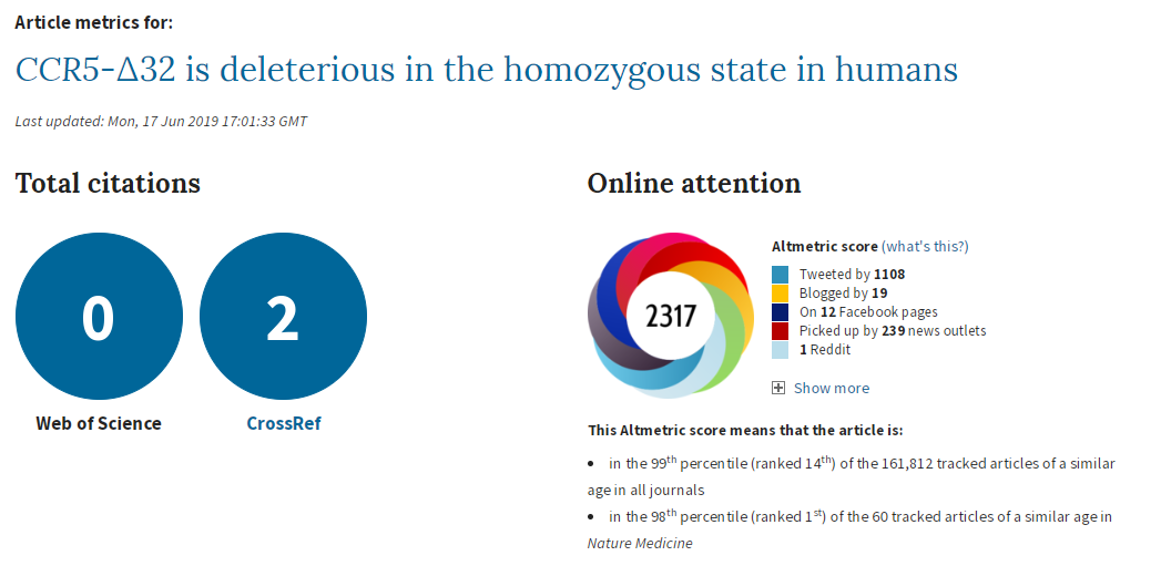
To recap, a couple of weeks ago a paper by Xinzhu (April) Wei & Rasmus Nielsen of the University of California was published, claiming that a deletion in the CCR5 gene increased mortality (in white people of British ancestry in UK Biobank). I had some issues with the paper, which I posted here. My tweets got more attention than anything I’d posted before. I’m pretty sure they got more attention than my published papers and conference presentations combined. ¯\_(ツ)_/¯

The CCR5 gene is topical because, as the paper states in the introduction:

In late 2018, a scientist from the Southern University of Science and Technology in Shenzhen, Jiankui He, announced the birth of two babies whose genomes were edited using CRISPR

To be clear, gene-editing human babies is awful. Selecting zygotes that don’t have a known, life-limiting genetic abnormality may be reasonable in some cases, but directly manipulating the genetic code is something else entirely. My arguments against the paper did not stem from any desire to protect the actions of Jiankui He, but to a) highlight a peer review process that was actually pretty awful, b) encourage better use of UK Biobank genetic data, and c) refute an analysis that seemed likely biased.

This paper has received an incredible amount of attention. If it is flawed, then poor science is being heavily promoted. Apart from the obvious problems with promoting something that is potentially biased, others may try to do their own studies using this as a guideline, which I think would be a mistake.

I’ll quickly recap the initial problems I had with the paper (excluding the things that were easily solved by reading the online supplement), then go into what I did to try to replicate the paper’s results. I ran some additional analyses that I didn’t post on Twitter, so I’ll include those results too.

Full disclosure: in addition to tweeting to me, Rasmus and I exchanged several emails, and they ran some additional analyses. I’ll try not to talk about any of these analyses as it wasn’t my work, but, if necessary, I may mention pertinent bits of information.

I should also mention that I’m not a geneticist. I’m an epidemiologist/statistician/evidence synthesis researcher who for the past year has been working with UK Biobank genetic data in a unit that is very, very keen on genetic epidemiology. So while I’m confident I can critique the methods for the main analyses with some level of expertise, and have spent an inordinate amount of time looking at this paper in particular, there are some things where I’ll say I just don’t know what the answer is.

I don’t think I’ll write a formal response to the authors in a journal – if anyone is going to, I’ll happily share whatever information you want from my analyses, but it’s not something I’m keen to do myself.

All my code for this is here.

The Issues

Not accounting for relatedness

Not accounting for relatedness (i.e. related people in a sample) is a problem. It can bias genetic analyses through population stratification or familial structure, and can be easily dealt with by removing related individuals in a sample (or fancy analysis techniques, e.g. Bolt-LMM). The paper ignored this and used everyone.

Quality control

Quality control (QC) is also an issue. When the IEU at the University of Bristol was QCing the UK Biobank genetic data, they looked for sex mismatches, sex chromosome aneuploidy (having sex chromosomes different to XX or XY), and participants with outliers in heterozygosity and missing rates (yeah, ok, I don’t have a good grasp on what this means, but I see it as poor data quality for particular individuals). The paper ignored these too.

Ancestry definition

The paper states it looks at people of “British ancestry”. Judging by the number in participants in the paper and the reference they used, the authors meant “white British ancestry”. I feel this should have been picked up on in peer review, since the terms are different. The Bycroft article referenced uses “white British ancestry”, so it would have certainly been clearer sticking to that.

Covariable choice

The main analysis should have also been adjusted for all principal components (PCs) and centre (where participants went to register with UK Biobank). This helps to control for population stratification, and we know that UK Biobank has problems with population stratification. I thought choosing variables to include as covariables based on statistical significance was discouraged, but apparently I was wrong. Still, I see no plausible reason to do so in this case – principal components represent population stratification, population stratification is a confounder of the association between SNPs and any outcome, so adjust for them. There are enough people in this analysis to take the hit.

The analysis

I don’t know why the main analysis was a ratio of the crude mortality rates at 76 years of age (rather than a Cox regression), and I don’t know why there are no confidence intervals (CIs) on the estimate. The CI exists, it’s in the online supplement. Peer review should have had problems with this. It is unconscionable that any journal, let alone a top-tier journal, would publish a paper when the main result doesn’t have any measure of the variability of the estimate. A P value isn’t good enough when it’s a non-symmetrical error term, since you can’t estimate the standard error.

So why is the CI buried in an additional file when it would have been so easy to put it into the main text? The CI is from bootstrapping, whereas the P value is from a log-rank test, and the CI of the main result crosses the null. The main result is non-significant and significant at the same time. This could be a reason why the CI wasn’t in the main text.

It’s also noteworthy that although the deletion appears strongly to be recessive (only has an effect is both chromosomes have the deletion), the main analysis reports delta-32/delta-32 against +/+, which surely has less power than delta-32/delta-32 against +/+ or delta-32/+. The CI might have been significant otherwise.

I think it’s wrong to present one-sided P values (in general, but definitely here). The hypothesis should not have been that the CCR5 deletion would increase mortality; it should have been ambivalent, like almost all hypotheses in this field. The whole point of the CRISPR was that the babies would be more protected from HIV, so unless the authors had an unimaginably strong prior that CCR5 was deleterious, why would they use one-sided P values? Cynically, but without a strong reason to think otherwise, I can only imagine because one-sided P values are half as large as two-sided P values.

The best analysis, I think, would have been a Cox regression. Happily, the authors did this after the main analysis. But the full analysis that included all PCs (but not centre) was relegated to the supplement, for reasons that are baffling since it gives the same result as using just 5 PCs.

Also, the survival curve should have CIs. We know nothing about whether those curves are separate without CIs. I reproduced survival curves with a different SNP (see below) – the CIs are large.

I’m not going to talk about the Hardy-Weinburg Equilibrium (HWE, inbreeding) analysis– it’s still not an area I’m familiar with, and I don’t really think it adds much to the analysis. There are loads of reasons why a SNP might be out of HWE – dying early is certainly one of them, but it feels like this would just be a confirmation of something you’d know from a Cox regression.

Replication Analyses

I have access to UK Biobank data for my own work, so I didn’t think it would be too complex to replicate the analyses to see if I came up with the same answer. I don’t have access to rs62625034, the SNP the paper says is a great proxy of the delta-32 deletion, for reasons that I’ll go into later. However, I did have access to rs113010081, which the paper said gave the same results. I also used rs113341849, which is another SNP in the same region that has extremely high correlation with the deletion (both SNPs have R² values above 0.93 with rs333, which is the rs ID for the delta-32 deletion). Ideally, all three SNPs would give the same answer.

First, I created the analysis dataset:

Grabbed age, sex, centre, principal components, date of registration and date of death from the UK Biobank phenotypic data
Grabbed the genetic dosages of rs113010081 and rs113341849 from the UK Biobank genetic data
Grabbed the list of related participants in UK Biobank, and our usual list of exclusions (including withdrawals)
Merged everything together, estimating the follow-up time for everyone, and creating a dummy variable of death (1 for those that died, 0 for everyone else) and another one for relateds (0 for completely related people, 1 for those I would typically remove because of relatedness)
Dropped the standard exclusions, because there aren’t many and they really shouldn’t be here
I created dummy variables for the SNPs, with 1 for participants with two effect alleles (corresponding to a proxy for having two copies of the delta-32 deletion), and 0 for everyone else
I also looked at what happened if I left the dosage as 0, 1 or 2, but since there was no evidence that 1 was any different from 0 in terms of mortality, I only reported the 2 versus 0/1 results

I conducted 12 analyses in total (6 for each SNP), but they were all pretty similar:

Original analysis: time = study time (so x-axis went from 0 to 10 years, survival from baseline to end of follow-up), with related people included, and using age, sex, principal components and centre as covariables
Original analysis, without relateds: as above, but excluding related people
Analysis 2: time = age of participant (so x-axis went from 40 to 80 years, survival up to each year of life, which matches the paper), with related people included, and using sex, principal components and centre as covariables
Analysis 2, without relateds: as above, but excluding related people
Analysis 3: as analysis 2, but without covariables
Analysis 3, without relateds: as above, but excluding related people

With this suite of analyses, I was hoping to find out whether:

either SNP was associated with mortality
including covariables changed the results
the time variable changed the results, and d) whether including relateds changed the results

Results

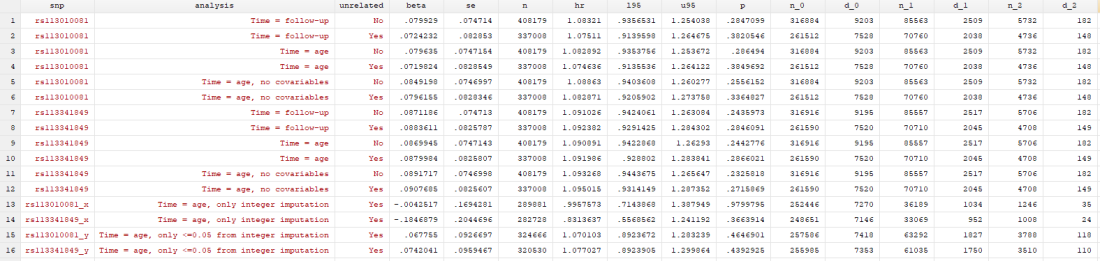
I found… Nothing. There was very little evidence the SNPs were associated with mortality (the hazard ratios, HRs, were barely different from 1, and the confidence intervals were very wide). There was little evidence including relateds or more covariables, or changing the time variable, changed the results.

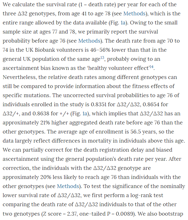
Here’s just one example of the many survival curves I made, looking at delta-32/delta-32 (1) versus both other genotypes in unrelated people only (not adjusted, as Stata doesn’t want to give me a survival curve with CIs that is also adjusted) – this corresponds to the analysis in row 6.

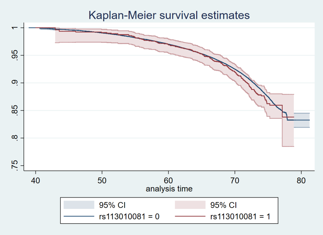
You’ll notice that the CIs overlap. A lot. You can also see that both events and participants are rare in the late 70s (the long horizontal and vertical stretches) – I think that’s because there are relatively few people who were that old at the end of their follow-up. Average follow-up time was 7 years, so to estimate mortality up to 76 years, I imagine you’d want quite a few people to be 69 years or older, so they’d be 76 at the end of follow-up (if they didn’t die). Only 3.8% of UK Biobank participants were 69 years or older.

In my original tweet thread, I only did the analysis in row 2, but I think all the results are fairly conclusive for not showing much.

In a reply to me, Rasmus stated:

This is the claim that turned out to be incorrect:

Never trust data that isn’t shown – apart from anything else, when repeating analyses and changing things each time, it’s easy to forget to redo an extra analysis if the manuscript doesn’t contain the results anywhere.

This also means I couldn’t directly replicate the paper’s analysis, as I don’t have access to rs62625034. Why not? I’m not sure, but the likely explanation is that it didn’t pass the quality control process (either ours or UK Biobank’s, I’m not sure).

SNPs

I’ve concluded that the only possible reason for a difference between my analysis and the paper’s analysis is that the SNPs are different. Much more different than would be expected, given the high amount of correlation between my two SNPs and the deletion, which the paper claims rs62625034 is measuring directly.

One possible reason for this is the imputation of SNP data. As far as I can tell, neither of my SNPs were measured directly, they were imputed. This isn’t uncommon for any particular SNP, as imputation of SNP data is generally very good. As I understand it, genetic code is transmitted in blocks, and the blocks are fairly steady between people of the same population, so if you measure one or two SNPs in a block, you can deduce the remaining SNPs in the same block.

In any case there is a lot of genetic data to start with – each genotyping chip measures hundred of thousands of SNPs. Also, we can measure the likely success rate of the imputation, and SNPs that are poorly imputed (for a given value of “poorly”) are removed before anyone sees them.

The two SNPs I used had good “info scores” (around 0.95 I think – for reference, we dropped all SNPs with an info score of less than 0.3 for SNPs with minor allele frequencies similar), so we can be pretty confident in their imputation. On the other hand, rs62625034 was not imputed in the paper, it was measured directly. That doesn’t mean everyone had a measurement – I understand the missing rate of the SNP was around 3.4% in UK Biobank (this is from direct communication with the authors, not from the paper).

But. And this is a weird but that I don’t have the expertise to explain, the imputation of the SNPs I used looks… well… weird. When you impute SNP data, you impute values between 0 and 2. They don’t have to be integer values, so dosages of 0.07 or 1.5 are valid. Ideally, the imputation would only give integer values, so you’d be confident this person had 2 mutant alleles, and this person 1, and that person none. In many cases, that’s mostly what happens.

Non-integer dosages don’t seem like a big problem to me. If I’m using polygenic risk scores, I don’t even bother making them integers, I just leave them as decimals. Across a population, it shouldn’t matter, the variance of my final estimate will just be a bit smaller than it should be. But for this work, I had to make the non-integer dosages integers, so anything less than 0.5 I made 0, anything 0.5 to 1.5 was 1, and anything above 1.5 was 2. I’m pretty sure this is fine.

Unless there’s more non-integer doses in one allele than the other.

rs113010081 has non-integer dosages for almost 14% of white British participants in UK Biobank (excluding relateds). But the non-integer dosages are not distributed evenly across dosages. No. The twos has way more non-integer dosages than the ones, which had way more non-integer dosages than the zeros.

In the below tables, the non-integers are represented by being missing (a full stop) in the rs113010081_x_tri variable, whereas the rs113010081_tri variable is the one I used in the analysis. You can see that of the 4,736 participants I thought had twos, 3,490 (73.69%) of those actually had non-integer dosages somewhere between 1.5 and 2.

What does this mean?

I’ve no idea.

I think it might mean the imputation for this region of the genome might be a bit weird. rs113341849 has the same pattern, so it isn’t just this one SNP.

But I don’t know why it’s happened, or even whether it’s particularly relevant. I admit ignorance – this is something I’ve never looked for, let alone seen, and I don’t know enough to say what’s typical.

I looked at a few hundred other SNPs to see if this is just a function of the minor allele frequency, and so the imputation was naturally just less certain because there was less information. But while there is an association between the minor allele frequency and non-integer dosages across dosages, it doesn’t explain all the variance in the estimate. There were very few SNPs with patterns as pronounced as in rs113010081 and rs113341849, even for SNPs with far smaller minor allele frequencies.

Does this undermine my analysis, and make the paper’s more believable?

I don’t know.

I tried to look at this with a couple more analyses. In the “x” analyses, I only included participants with integer values of dose, and in the “y” analyses, I only included participants with dosages < 0.05 from an integer. You can see in the results table that only using integers removed any effect of either SNP. This could be evidence that the imputation having an effect, or it could be chance. Who knows.

rs62625034

rs62625034 was directly measured, but not imputed, in the paper. Why?

It’s possibly because the SNP isn’t measuring what the probe meant to measure. It clearly has a very different minor allele frequency in UK Biobank (0.1159) than in the GO-ESP population (~0.03). The paper states this means it’s likely measuring the delta-32 deletion, since the frequencies are similar and rs62625034 sits in the deletion region. This mismatch may have made it fail quality control.

But this raises a couple of issues. First is whether the missingness in rs62625034 is a problem – is the data missing completely at random or not missing at random. If the former, great. If the latter, not great.

The second issue is that rs62625034 should be measuring a SNP, not a deletion. In people without the deletion, the probe could well be picking up people with the SNP. The rs62625034 measurement in UK Biobank should be a mixture between the deletion and a SNP. The R² between rs62625034 and the deletion is not 1 (although it is higher than for my SNPs – again, this was mentioned in an email to me from the authors, not in the paper), which could happen if the SNP is picking up more than the deletion.

The third issue, one I’ve realised only just now, is that previous research has shown that rs62625034 is not associated with lifespan in UK Biobank (and other datasets). This means that maybe it doesn’t matter that rs62625034 is likely picking up more than just the deletion.

Peter Joshi, author of the article, helpfully posted these tweets:

If I read this right, Peter used UK Biobank (and other data) to produce the above plot showing lots of SNPs and their association with mortality (the higher the SNP, the more it affects mortality).

Not only does rs62625034 not show any association with mortality, but how did Peter find a minor allele frequency of 0.035 for rs62625034 and the paper find 0.1159? This is crazy. A minor allele frequency of 0.035 is about the same as the GO-ESP population, so it seems perfectly fine, whereas 0.1159 does not.

I didn’t clock this when I first saw it (sorry Peter), but using the same datasets and getting different minor allele frequencies is weird. Properly weird. Like counting the number of men and women in a dataset and getting wildly different answers. Maybe I’m misunderstanding, it wouldn’t be the first time – maybe the minor allele frequencies are different because of something else. But they both used UK Biobank, so I have no idea how.

I have no answer for this. I also feel like I’ve buried the lead in this post now. But let’s pretend it was all building up to this.

Conclusion

This paper has been enormously successful, at least in terms of publicity. I also like to think that my “post-publication peer review” and Rasmus’s reply represents a nice collaborative exchange that wouldn’t have been possible without Twitter. I suppose I could have sent an email, but that doesn’t feel as useful somehow.

However, there are many flaws with the paper that should have been addressed in peer review. I’d love to ask the reviewers why they didn’t insist on the following:

The sample should be well defined, i.e. “white British ancestry” not “British ancestry”
Standard exclusions should be made for sex mismatches, sex chromosome aneuploidy, participants with outliers in heterozygosity and missing rates, and withdrawals from the study (this is important to mention in all papers, right?)
Relatedness should either be accounted for in the analysis (e.g. Bolt-LMM) or related participants should be removed
Population stratification should be both addressed in the analysis (maximum principal components and centre) and the limitations
All effect estimates should have confidence intervals (I mean, come on)
All survival curves should have confidence intervals (ditto)
If it’s a survival analysis, surely Cox regression is better than ratios of survival rates? Also, somewhere it would be useful to note how many people died, and separately for each dosage
One-tailed P values need a huge prior belief to be used in preference to two-tailed P values
Over-reliance on P values in interpretation of results is also to be avoided
Choice of SNP, if you’re only using one SNP, is super important. If your SNP has a very different minor allele frequency from a published paper using a very similar dataset, maybe reference it and state why that might be. Also note if there is any missing data, and why that might be ok
When there is an online supplement to a published paper, I see no legitimate reason why “data not shown” should ever appear
Putting code online is wonderful. Indeed, the paper has a good amount of transparency, with code put on github, and lab notes also put online. I really like this.

So, do I believe “CCR5-∆32 is deleterious in the homozygous state in humans”?

No, I don’t believe there is enough evidence to say that the delta-32 deletion in CCR-5 affects mortality in people of white British ancestry, let alone people of other ancestries.

I know that this post has likely come out far too late to dam the flood of news articles that have already come out. But I kind of hope that what I’ve done will be useful to someone.

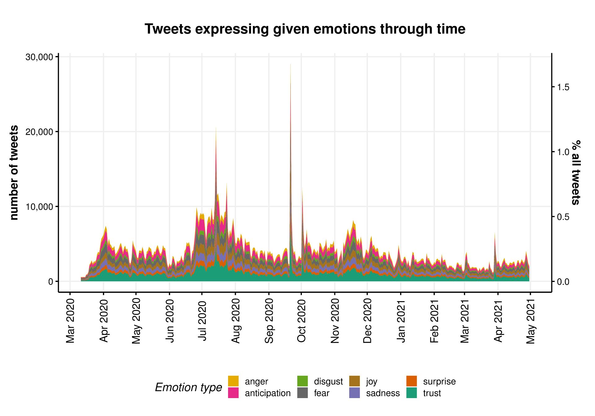
Conference time at the MRC Integrative Epidemiology Unit!

Posted on July 8, 2019 by lindsey.pike

Dr Jack Bowden, Programme Leader

Follow Jack on Twitter

Every two years my department puts on a conference on the topic of Mendelian Randomization (MR), a field that has been pioneered by researchers in Bristol over the last two decades. After months of planning, including finding a venue, inviting speakers from around the world and arranging the scientific programme, it’s a week and a half to go and we’re almost there!

But what is Mendelian Randomization research all about I hear you ask? Are you sure you want to know? Please read on but understand there is no going back…..

Are you sure you want to know about Mendelian Randomisation?

Have you ever had the feeling that something wasn’t quite right, that you are being controlled in some way by a higher force?

Well, it’s true. We are all in The Matrix. Like it or not, each of us has been recruited into an experiment from the moment we were born. Our genes, which are given to us by our parents at the point of conception, influence every aspect of our lives: how much we eat, sleep, drink, weigh, smoke, study, worry and play. The controlling effect is cleverly very small, and scientists only discovered the pattern by taking measurements across large populations, so as individuals we generally don’t notice. But the effect is real, very real!

How can we fight back?

We cannot escape The Matrix, but we can fight back by extracting knowledge from this unfortunate experiment we find ourselves in and using it for society’s advantage. For example, if we know that our genes predict 1-2% of variation in Low-Density Lipoprotein cholesterol (LDL-c – the ‘bad’ cholesterol) in the population, we can see if genes known to predict LDL-c also predict later life health outcomes in a group of individuals such as an increased risk of heart disease. If they do, then it provides strong evidence that reducing LDL-c will reduce heart disease risk, and we can then take steps to act. This is, in essence, the science of Mendelian randomization. See here for a nice animation of the method by our Unit director, George Davey Smith – our Neo if you like.

An example of the mathematical framework that leads to our analysis (honest)

Mendelian randomization is very much a team effort, involving scientists with expertise across many disciplines. My role, as a statistician and data scientist is to provide the mathematical framework to ensure the analysis is performed in a rigorous and reliable manner.

We start by drawing a diagram that makes explicit the assumptions our analysis rests on. The arrows show which factors influence which. In our case we must assume that a set of genes influence LDL-c, and can only influence heart disease risk through LDL-c. We can then translate this diagram into a system of equations that we apply to our data.

The great thing about Mendelian randomization is that, even when many other factors jointly influence LDL-c and heart disease risk, the Mendelian randomization approach should still work.

Recently, the validity of the Mendelian randomization approach has been called into question due to the problem of pleiotropy. In our example this would be when a gene affects heart disease through a separate unmodelled pathway.

This can lead to bias in the analysis and therefore misleading results. My research is focused on novel methods that try to overcome the issue of pleiotropy, by detecting and adjusting for its presence in the analysis. For further details please see this video.

The MR Data challenge

At this year’s conference we are organising an MR Data Challenge, to engage conference participants in exploring and developing innovative approaches to Mendelian randomization using a publicly available data set. At a glance, the data comprises information on 150 genes and their association with

118 lipid measurements (LDL cholesterol)
7 health outcomes (including type II diabetes)

Eight research teams have submitted an entry to the competition, to describe how they would analyse the data and the conclusions they would draw. The great thing about these data is that the information on all 118 lipid traits simultaneously assessed to improve the robustness of the Mendelian randomization analysis.

Genetic data can help us understand how to resolve population health issues. Image credit: www.genome.gov

A key aim of the session is to bring together data scientists with experts from the medical world to comment on and debate the results. We will publish all of the computer code online so that anyone can re-run the analyses. In the future, we hope to add further data to this resource and for many new teams to join the party with their own analysis attempt.

Please come and join us at the MR conference in Bristol, 17-19 July, it promises to be epic!

Category: methods